Meta-Learning Generative Adversarial Networks for Extrapolating Nonlinear Dynamic Stochastic Systems.
Case Study: Price Forecasting of Volatile Assets for use in Algorithmic Trading.
Abstract
Financial markets are complex systems and are not easily modelled with continuous functions. Some methods exist which parametrize market conditions based on assumptions about trader behaviour, but these fall short when the factors influencing these behavioral assumptions change. Modelling financial markets as non-linear dynamic stochastic systems circumvents these shortcomings but imposes new limitations as such systems are not easily modelled. A meta-learning generative adversarial network is herein proposed to predict future-states of these systems and it is evaluated on real (price of bitcoin) and generated data.
1. Introduction
1.1 Market Modeling Background
Financial markets, in particular cryptocurrencies which are highly volatile, have random walk properties. Furthermore, the fundamental properties which affect an asset’s price are many and attempts to measure and model them might result in changes escaping the scope of the measurement. Despite these random walk properties, the change in price of an asset observes a constant distribution so the price of an asset can be effectively modelled as a stochastic process. The famous Black-Scholes equation describes the price of an asset as one that “follows a geometric Brownian motion with constant drift and constant volatility” (Zhang 2) which satisfies this differential equation.
Where S is price and W is a Wiener process of Brownian motion, and μ and σ are constants denoting drift and volatility respectively. The Black-Scholes equation is known to have some limitations, however, notably its assumption of market volatility as a constant property.
In their 2000 paper, Cars H. Hommes models financial markets as a nonlinear adaptive belief system with multiple variables relating to types of investors and price vectors; stating, “evolutionary adaptive systems with heterogeneous agents using competing trading strategies [are] a natural nonlinear world full of homoclinic bifurcations and strange attractors” (Hommes 6).
Where F is a nonlinear mapping, Xt is a vector of prices, njtis the fraction or weight of investors of type h, λ is a vector of parameters and δtand ϵt are noise terms (Hommes 6).
1.2 Limits of Structured Market Models
A problem with these solutions is the assumption of some market structure. Particularly in an adaptive belief market, a structure which may exist at one time will likely not exist in another. Abstractions can be made through which an analytical solution might be reached but this could ultimately prove fruitless in an efficient market. The model must change as quickly if not faster than the market.
Where X is a vectorized sample of S and Θk is a set of parameters.
1.3 Learning-Based Problem Framing
Assuming the distribution of possible future states to be finite, the price of an asset can be described as a finite state system for which there is a function which precisely determines future states from information of current and past states. The function described by phi and theta can accurately model the system while the properties (unknown to the observer) of the system theta trains on remain constant. By parametrizing the system as a neural network with millions of parameters, the proposed model aims to assume the least possible about market structures and dynamics. These will be learned by the model and will remain unknown.
Be it slippage or localized panic and euphoria, the price of a volatile asset often oscillates around a “true” price in what will be henceforth referred to as noise.
These high frequency undulations in price can not be profited from because of the long time it takes to enter and exit trades; primarily resulting from request-response lag and time to fill orders. This can be mitigated by placing only market orders, but this might result in slippage which in turn affects the accuracy of a model.
2. Concept
2.1 Forecasting Objective
As a solution to stochastic, deterministic system with unknown inputs, a neural network is developed which can learn how the expected distribution of future data relates to the known distribution of present and past data. This way, a likely prediction can be used to implement trades. This has the added benefit of not relying on precision as it is likely that the future price of an asset would immediately diverge from the predicted price the moment a trade was enacted on the predicted information. Generative adversarial networks learn to replicate the stochasticity of data (Isola 7) and as such are appropriate for this solution (7).
(Eq. 7 Isola 3, Eq. 8 Finn 3)
Where Dk is a windowed set of price data samples between t and t-ws (ws is window size) subsampled from the set containing all of the asset’s price data, Θk is its corresponding set of parameters, G is a generator which attempts to produce “real” data, and D is a discriminator which trains to distinguish “real” data from that produced by the generator.
2.2 Task-Level Adaptation
For temporal stability between predictions, the network’s previous prediction is also input. In accordance with the adaptive efficient market hypothesis, the network must be routinely actualized such that it keeps up with the changing system. This is facilitated by the meta learning model described in (8) which ensures the model can quickly and effectively train on new tasks as they arise; changing market conditions are analogous to new tasks. Finally, the proposed model takes the form of a nonlinear mapping function which maps a vector of parameters Θ, a windowed set of price observations D ,and its previous prediction Xt-1 to a new price prediction Xt (6).
3. Proof of Concept
3.1 Distribution of Candle-Level Changes
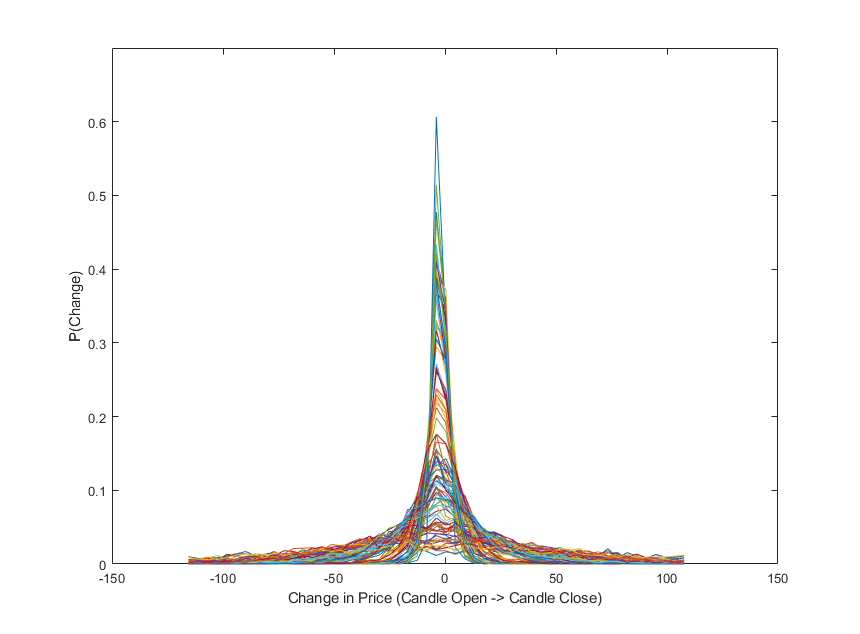
Imperative to the design of this neural network is that the change in price between candles can be reasonably described as a stochastic process, independent of market conditions. To validate this assertion, one hundred samples of two thousand candles were randomly selected from the price of Bitcoin between the years 2021 and 2022; these years were selected because they had constant and reasonable trading volume throughout. Probability distributions were then created for each of these samples using histograms, and events with a probability of occurrence below 1e-3 were discarded.
Figure 1 shows the probability distributions for the one hundred samples. With ten thousand samples like the ones used for figure 1, subsample mean was determined to have mean 0.0107 and standard deviation 0.7823. Subsample standard deviation was found to have mean 30.7794 with standard deviation 24.4113. The extent to which the assertion holds true is ultimately determined by the model’s performance, but from figure one, it can at least be concluded that the dataset does observe a relatively constant mean around zero with reasonable probability that change of price is less than twenty-five dollars, for any subsample.
3.2 Spectral Variation Across Market Regimes
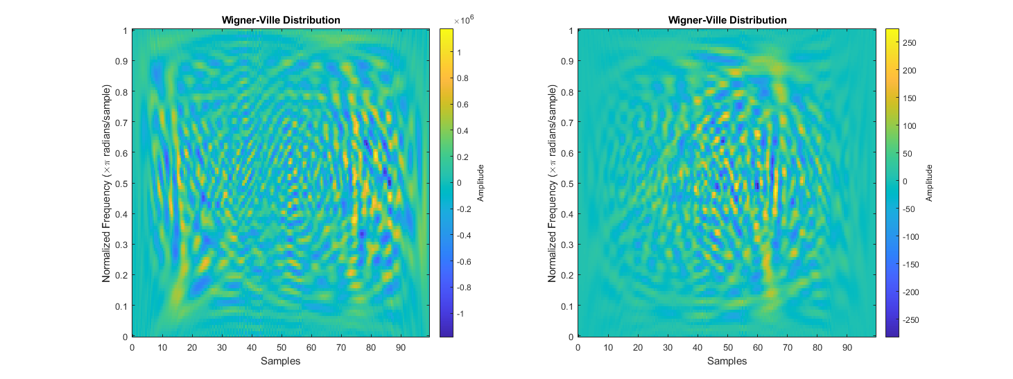
Despite similarities in distribution, market conditions do influence changes in price, and this is evident when analyzing the spectral content of a sample. To illustrate the effect of market conditions on a sample’s spectral content, one high energy sample, and one low energy sample were selected for comparison. The samples’ energy was calculated as the sum of the sample’s squared fast Fourier transform; from a set of a hundred samples of a hundred candles, the samples with the highest and lowest energy readings were selected. The high-energy event corresponded to a high-volume trading scenario where within the hundred sampled candles, price changed by over one thousand USD. In the low-energy event, change in price across the entire sample was less than fifty USD.
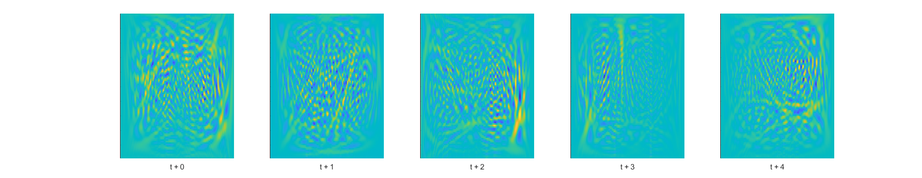
3.3 Continuity Across Consecutive Windows
4. Implementation
4.1 Wavelet Input Construction
The price of an asset is observed at a regular frequency and samples having n observations are created. To reveal underlying trends, and encode inputs with frequency-information, samples are upscaled by the continuous wavelet transform (cwt).
4.2 Adversarial Objective and Loss Formulation
For the network to learn system properties unique to the sample time, a set of wavelet-transformed signals is created by retaining the upscaled samples for a specified window. The meta learning model then learns features between different sample times (with varying market conditions) and determines which are relevant when faced with a “new” system state. Generative-Adversarial networks are implemented because they learn to replicate a dataset’s stochasticity which is desirable when the system has random-walk properties but maintains relatively uniform change-of-state distributions.
Instead of the network’s previous prediction, during training the expected output plus a noise vector ζ is input. Additionally, a noise set Dz and noise vector z is input so the adversarial network does not produce deterministic outputs (Isola 3). Equations 13-15 are the equations detailed in Isola et Al’s Image-To-Image Translation with Conditional Adversarial Networks (7) modified to such that they accept sets of wavelets transformed data (12) as inputs. These provide a general overview of the network’s learning targets though the implemented architecture contains several sublayers some of which have their own.
Where a sublayer has a unique learning target, its loss function is described in the section detailing that layer and the compounded loss function which replaces equation 16 is denoted by equation 35. During training however, equation 36 is used instead of 35 for its ease of implementation.
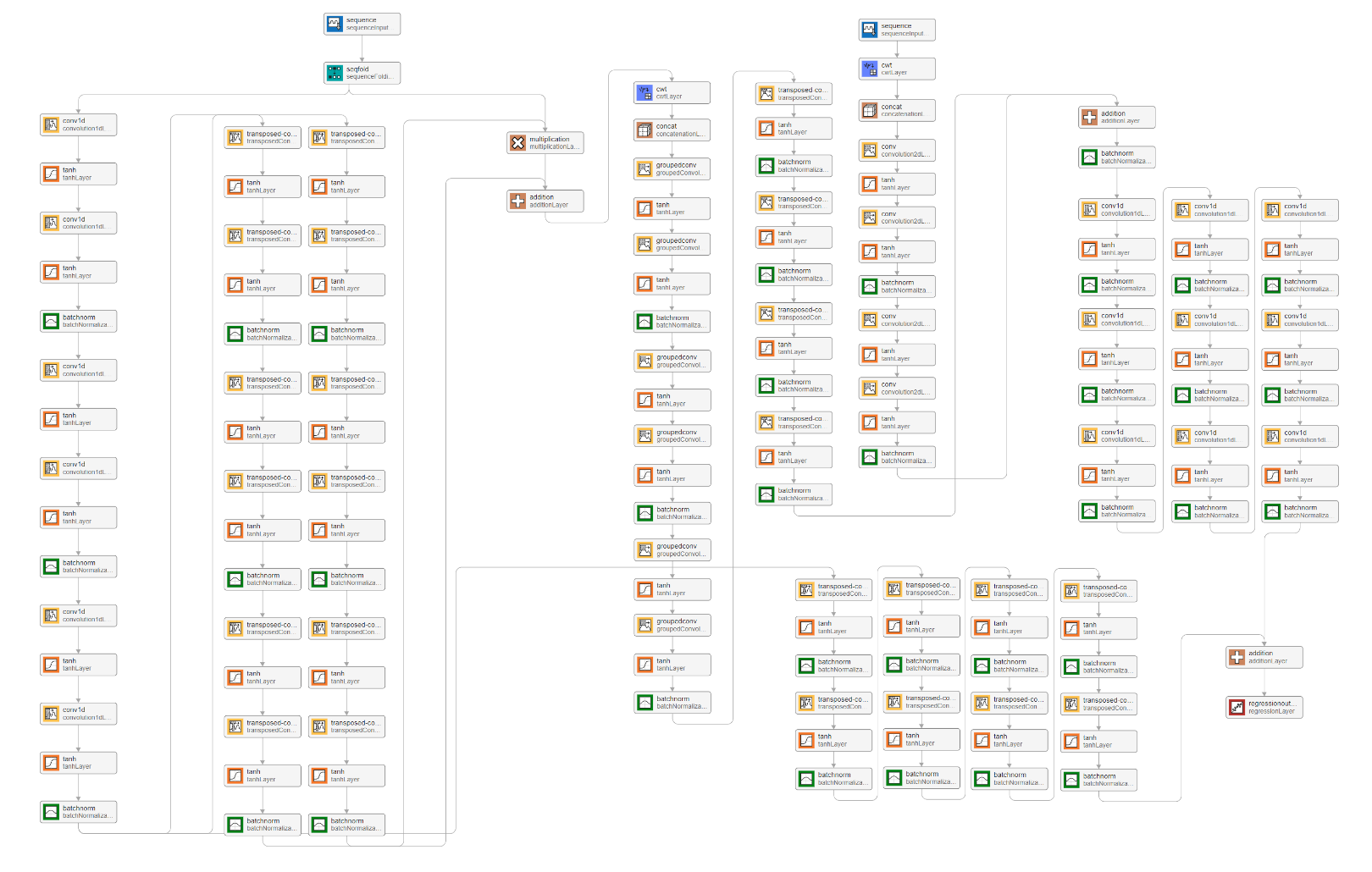
4.3 Generator Architecture
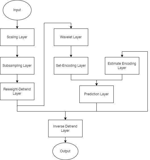
The implemented network is a generator-discriminator pair with several targets for learning. The generator is comprised of eight layers each with their own sublayers. In no order, the generator’s layers are a scaling layer, a subsampling layer, a reweighting and detrending layer, a wavelet layer, a set-encoding layer, an estimate-encoding layer, a prediction layer, and an inverse-detrending layer. The generator accepts one dimensional inputs of the sampled change in price signal, and outputs one dimensional extrapolated predictions of that same price signal. For temporal stability, the generator’s previous estimate is also input. While backpropagation is performed on all the layers simultaneously, loss is calculated for certain layers independently of the others before it is compounded for updating the gradients. This results in some changes to the loss functions detailed in equations 13 and 15.
The discriminator is essentially a condenser network trained with patch-Gan loss but since it accepts one dimensional samples of the price signal, its inputs undergo a transformation by the continuous wavelet transform before convolution. This will ensure that the samples the generator produce have similar frequency content to real samples.
4.4 Scaling Layer
This layer scales a large sample of candles and scales the data such that all values are approximately in the range between -1 and 1. The number of candles this layer accepts as input depends on subsample window size, number of subsamples, and overlap between subsamples and is calculated with equation 16.
Where x is a vector of candle data containing nCandles. At the time of writing, this layer scales samples by dividing each element by a scale factor; Scale factor is determined by fitting a normal distribution to X, then taking SF as the value corresponding to 0.95 on the cumulative distribution.
4.5 Subsampling Layer
The subsampling layer rearranges the scaling layer’s output into a two-dimensional array of dimensions [WindowSize, nSubsamples] whose rows each are a unique sample which overlaps the subsequent sample as dictated by the Overlap parameter. This layer is what converts a linear sample into a dataset sample and prepares the data for upscaling via the wavelet transform.
4.6 Reweight-Detrend Layer
Before data can be upscaled with the continuous wavelet transform, some steps must be taken to prevent loss of information and to maximize the accuracy of the final prediction. The continuous wavelet transform convolves a signal with a sliding wavelet at changing dilations to reveal the signal’s frequency information; each dilation corresponds with a specific wavelength. To focus the wavelet, transform on higher frequency oscillations, the continuous wavelet transform algorithm applies a detrending operation to the data before convolving with wavelets. However, it does not return information about the detrend which would later affect the network’s ability to predict future states.
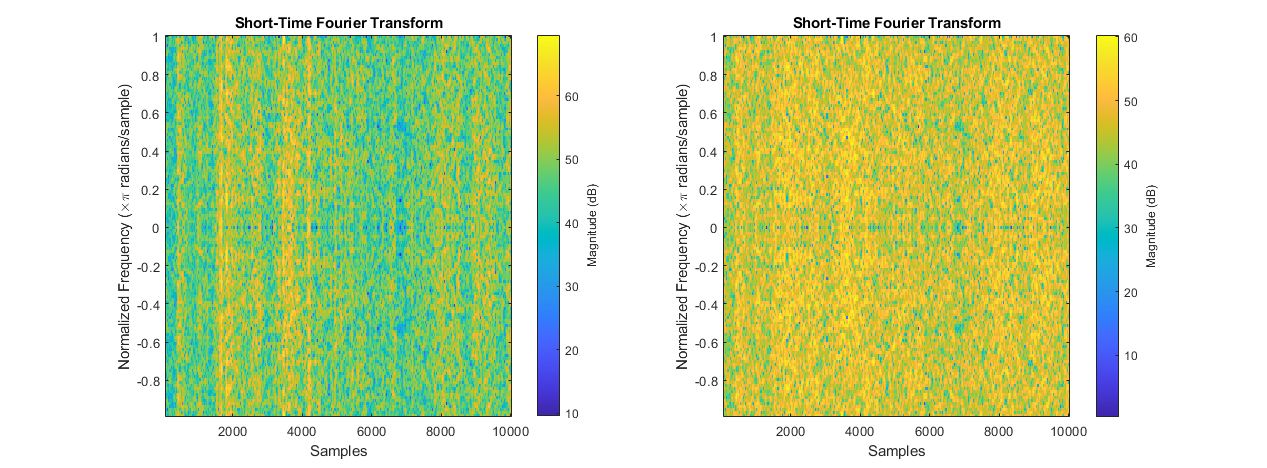
Furthermore, the dataset in question has random-walk properties which skew sample statistics and severely reduce the network’s accuracy in prediction. Figure 5 compares the short time Fourier transforms (STFT) of raw (left) and reweighted (right) price data. In the raw data’s STFT, some high energy bands can be seen which indicate the presence of outlying points of data. Samples which contain outlying datapoints have vastly different shapes from regular samples, often appearing as flat lines with one or two peaks. A reweighting operation is therefore necessary to remove or mitigate the effects of these outlying datapoints.
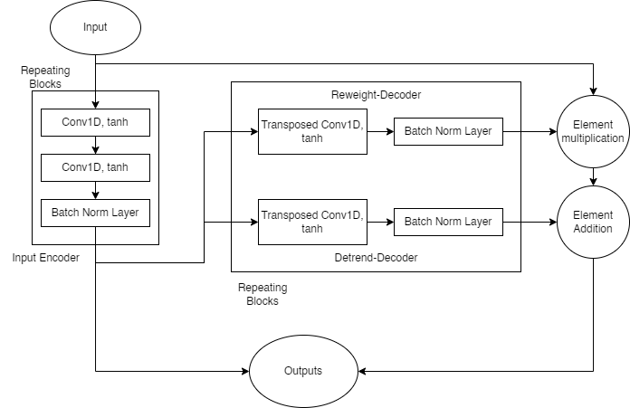
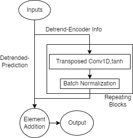
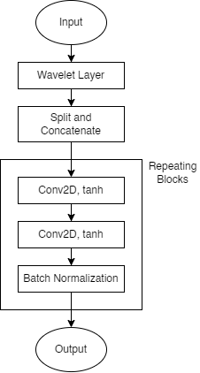
This reweight-detrend layer seeks to identify and mitigate the effects of outlying datapoints, while applying its own detrend to the data, and returning information about these operations for use in other layers. Subsampled data is first passed through an encoder whose output is then used to generate reweighting and detrending information in parallel. The subsampled data is then reweighted and detrended. As illustrated in figure 6, the encoder sublayer uses repeating blocks of two consecutive one dimensional convolutions with tanh activations, followed a batch normalization layer. The encoder sublayer’s output is stored for use in the inverse-detrend layer. The detrend-decoder and reweight-decoder sublayers have the same architecture, repeating blocks of transposed one-dimensional convolutions with tanh activations and batch normalization layers. The reweight-decoder’s output is then combined with the layer’s original input via element wise multiplication, then element-wise summed with the detrend-decoder’s output to produce this layer’s output.
The reweight-detrend layer has its own learning target, designed to optimize its performance with the rest of the network. This layer trains to minimize Huber loss between this layer’s output and an ideal output. The ideal output is empirically determined by reweighting the sample with Huber’s weight function then in series applying the continuous and inverse continuous wavelet transforms (See equation 29).
To generate ideal reference outputs for calculating loss, a scaled sample is reweighted with Huber’s weight function using a scaled residual. The residual is the absolute difference between an element and the sample’s median (eq 23), and the scale factor is the median absolute deviation of the sample, divided by 0.6745 (eq 24) which is the inverse of the coefficient used to compute Huber weight (eq 25). This method with 0.6475 as a coefficient has good performance/accuracy when identifying outlying datapoints (Akram et al.).
1.547|Xi|-1, otherwise}
δ|Xi - Yi| - 0.5δ2, otherwise}
(Equation 23-25, Akram et al. Equation 26, Beale et al.)
The Huber loss function used computes loss according to equation 26 and defaults to epsilon 1 (Beale et al. 1-759). It is beyond the scope of this investigation to change the value of epsilon, so the default value is used throughout. This loss function also sums loss across batches which satisfies one of the criteria for meta-learning detailed in equation eight.
4.7 Wavelet Layer
This layer upscales reweighted and detrended data by convolving it with a wavelet at different dilations, thus revealing some information about the signals’ frequency content. This layer converts batches of two-dimensional arrays of signals into batches of three-dimensional sets of the samples’ frequency information. The continuous wavelet transform algorithm is the one selected for its capacity to reveal lots of detail about a signal’s frequency content, and a morse wavelet is used for the convolution. The exact specifications of the wavelet are determined by the algorithm and are dependent on the sample’s window size.
4.8 Set-Encoding Layer
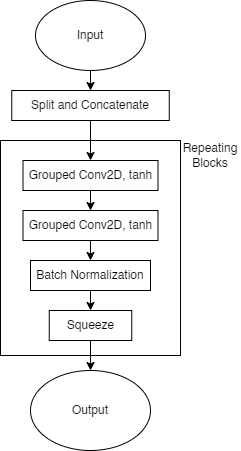
The set encoding layer uses grouped two-dimensional convolutions to extract features from sets of consecutive samples’ spectral content. This layer also splits the wavelet-layer output into its real and complex components and concatenates them along the fourth dimension. This is so model gradients are not complex valued. After splitting and concatenating the data, the set-encoding layer uses repeating blocks - each having two consecutive grouped two dimensional convolutions with tanh activations, and a batch normalization layer - to extract features from the set. For compatibility with other layers in the network which do not have as many dimensions to their data, the grouped convolutions ensure that the output from the repeating blocks has one singleton dimension, which is then removed by squeezing the data.
4.9 Estimate-Encoding Layer
For stability between consecutive predictions, this network also uses as input, its previous prediction. The previous estimate is stored within the network object during use and in training, the last, scaled, detrended input sample plus a noise vector is used. This layer calls the wavelet function to upscale the previous prediction for encoding. Besides the wavelet layer, the estimate-encoder’s architecture is like the set-encoding layer’s but designed to handle fewer dimensions. See appendix A for diagram.
4.10 Prediction Layer
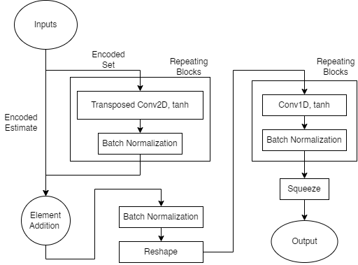
With the set and estimate encoders’ outputs as input, this layer predicts scaled and detrended future system states. In effect this layer is a transfer function which maps the encoders’ outputs to scaled and detrended future states (29). This layer has two decoders with the same convolution, batch norm architecture, operating at different dimensionalities.
This layer also has its own learning targets, which seek to ensure this layer’s output matches the reweighted-detrended extrapolation. Huber loss is calculated according to equation twenty-five, and its reference outputs are generated in the same method as for the reweight-detrend layer. It is important to note that the output is scaled by the scaling layer before reweighting and detrending.
Where Xset and Xestimate are the set and estimate encoding layers’ outputs respectively, ICWT and CWT are the inverse and continuous wavelet transforms, YSDT is the reweighted and detrended reference output as calculated by equation 29, and WHuber are Huber weights as calculated with equations 23 through 25.
4.11 Inverse-Detrend Layer
The final layer for this generator implementation, the inverse detrend layer uses information from the reweighting detrending layer to generate a vector which is then added to the prediction layer’s output to recover the signal’s underlying trend.
This layer uses repeating blocks of transposed one-dimensional convolutions, with hyperbolic tangent activations, and batch normalization layers to generate the trending vector. The vector is then added to the detrended prediction to recover the trended signal.
This layer also has its own learning targets which seek to minimize the error between this layer’s output and the scaled reference output. Like other layers with their own learning targets in this network, this layer’s loss is computed as the smooth L1 (Huber) loss between its output and a reference output. The reference output used for this layer’s loss function is the windowed sample, time shifted forward by a fixed extrapolation length. This sample is scaled by dividing it by a scale factor (as determined in equation 17). When generating training samples this is achieved with the scaling layer.
4.12 Compound Loss Function
Since gradients will be computed for the entire network simultaneously, each sublayer’s loss is compounded into a complete loss function which replaces equation 15. For ease of implementation, equation 36 is used instead of 35.
4.13 Discriminator Architecture
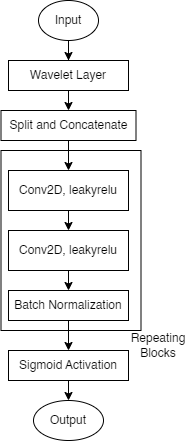
The discriminator for this architecture ensures the spectral content of a generated sample matches that of a real sample. It achieves this by obtaining the continuous wavelet transform of a sample followed by repeating blocks each containing two two-dimensional convolutions with leakyrelu activations, and a batch normalization layer. A sigmoid activation is then used to regularize this layer’s output between zero and one. Loss for this layer is calculated according to equation 15.
4.14 Considerations for Training and Evaluation
While training, gradients are computed for each sublayer individually, with respect to overall generator and discriminator loss as described by equation 14, with equation 36 replacing equation 15. In the gradient operation, both the set and estimate encoders are treated as one sublayer.
Gradients are computed with Adam, and each sublayer (including the discriminator) has its own learning parameters, average gradient, average squared gradient. Learn rates only vary between the generator and discriminator, though while evaluating this model both were kept the same.
This model was evaluated for its performance extrapolating nonlinear dynamic stochastic systems at varying extrapolation lengths at fixed window sizes, overlap between subsamples, and number of subsamples; ultimately, these parameters dictate the amount of system information available to the network.
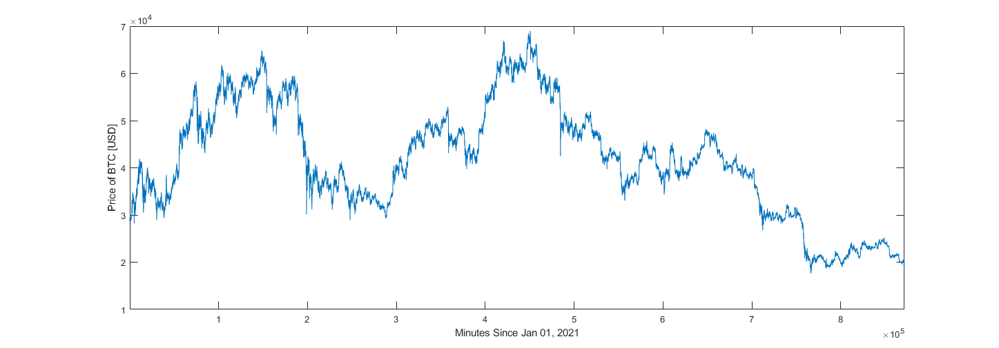
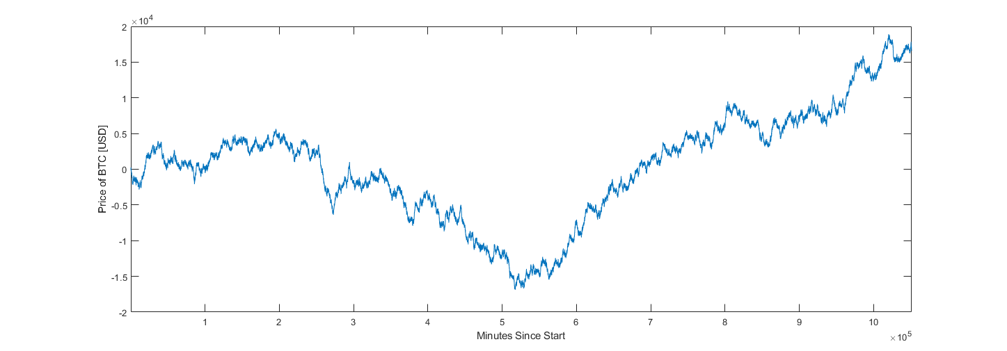
Evaluations were conducted on real and generated datasets. The price of Bitcoin between January 1, 2021, and October 1, 2022, sampled at one-minute intervals was queried from Binance’s online archives and is used as real data. Alternative datasets each containing approximately one million samples were generated according to equations 37 and 38 using 30 degrees of freedom.
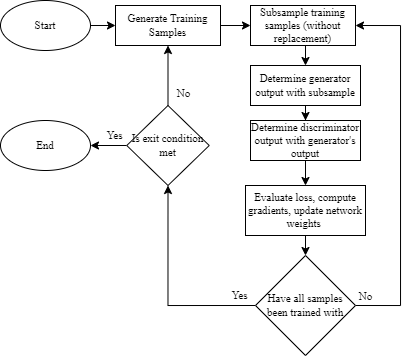
When evaluating the model’s performance relative its meta parameters (window size, extrapolation length, etc.) datasets were subsampled randomly five thousand times. To evaluate this model’s performance on a larger “real” dataset, a loop was created which would generate new samples from the dataset at every epoch. The idea being that the network would eventually have exposure to all the different market scenarios available in the dataset. Details of this loop are available in appendix A.
5. Evaluation
5.1 Extrapolation-Length Study
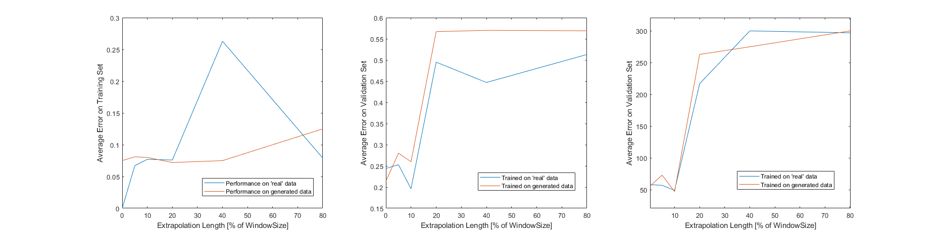
Hardware limitations restricted the metaparamers which could be feasibly evaluated, so the only parameters tested are those which describe the architecture in figure 11. Window size and overlap were set to 80 and 30 minutes respectively while the number of subsamples was 30. This model was evaluated at several extrapolation lengths and the results can be seen in figure 12. These agree with the assertion made in an earlier report which stated that the spectral content of a sample taken at time t + k ceases to be like that of the sample at time t, when k is approximately ten percent of the sample’s window size (Luna, 11). An extrapolation length of 80% was also tested though the discriminator’s layer sizes were increased considerably (for this test the discriminator had approximately 1.5x more learnable parameters than the generator). After 297 epochs with five thousand training samples, average error on the training set was 0.079 while average error on the validation set was 0.513. Training and validation sets were sampled separately from the ‘real’ dataset. The results obtained by increasing the discriminator’s layer sizes suggest that the discriminator’s role might be understated. Better results might be obtained by modifying the discriminator’s architecture. It should be noted that for figure 12, training concluded when average error was less than 0.08, or when 300 epochs had elapsed.
5.2 Synthetic-to-Real Transfer
It was also determined that when trained on data generated according to equations 37-39, the model exhibited similar performance on real data as when trained solely on real data. The assumptions about the system used to generate data are accurate.
5.3 Pre-Production Validation
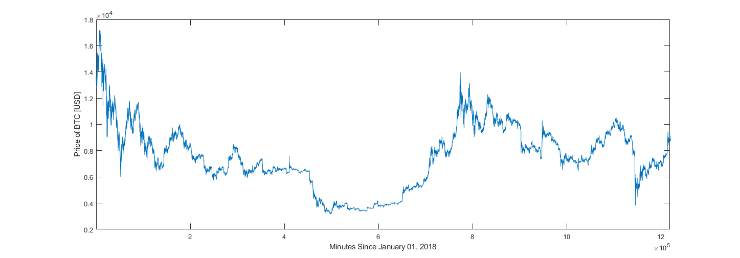
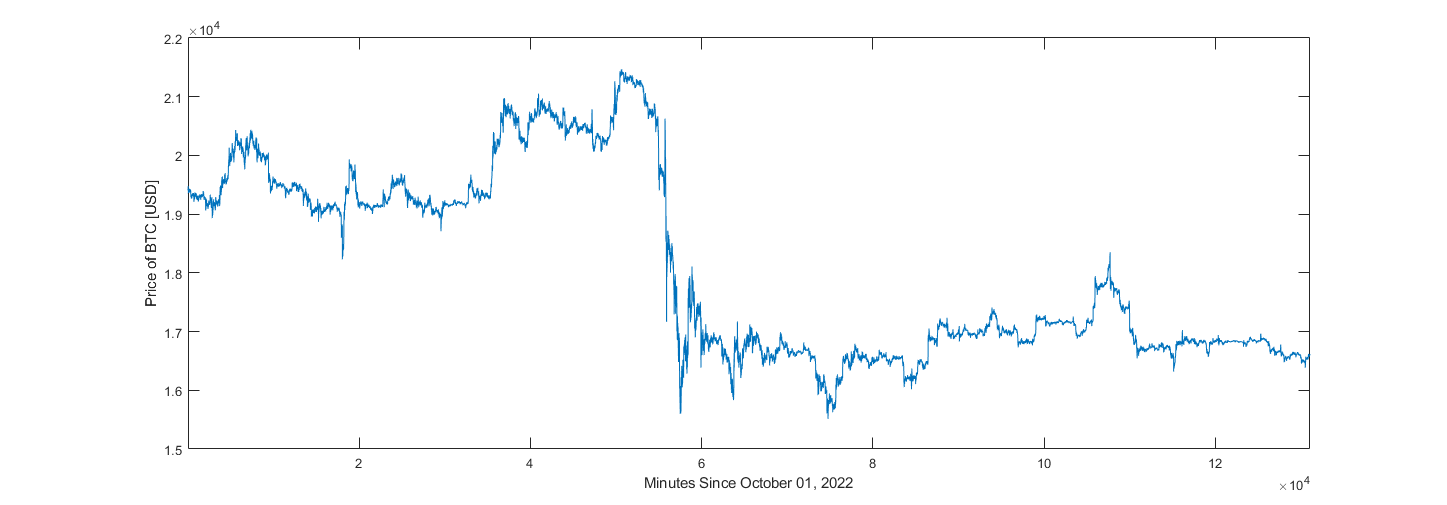
For pre-production validation (production being the training and deployment of this model for use in trading) this model was trained to extrapolate price data 20% of the sample’s window size forward, on one-minute candle data taken between January 1, 2018, and October 1, 2022. It was first attempted to have the training loop draw five thousand random samples from the price dataset after each epoch, though with the model and hyperparameters used for figure 12 the extrapolated values tended to zero. A slightly smaller dataset, containing ten thousand randomly selected samples was used to validate this model at 20% relative extrapolation length. After 410 epochs with ten thousand samples, average error on training data was 0.1355. Average errors on samples (not used in training) drawn randomly from training and validation datasets were 0.442 and 0.445 respectively. Validation dataset was data unavailable to the network during training; one minute candle data taken between October 1, 2022, and December 31, 2022.
![Figure 13 Reference [Blue] and Predicted [Orange] Samples from Training Set (and their cumulative sums)A line is drawn which marks the border between known and extrapolated values.](/src/images/meta-learning-trading-ai/image13.png)
![Figure 14 Reference [Blue] and Predicted [Orange] Samples from Validation Set (and their cumulative sums)A line is drawn which marks the border between known and extrapolated values.](/src/images/meta-learning-trading-ai/image14.png)
Appendix A: Additional Network Information
Estimate Encoding Layer Architecture Overview and “Production” Training Loop
Generator Layer Sizes During Evaluation
| Reweight-Detrend Layer [FilterSize nChannels nFilters] | ||||
| Input Encoder | Reweight Decoder | Detrend Decoder | ||
| Encoder Layers | ||||
| Set Encoder [FilterSizeX FilterSizeY nChannelsPerGroup nFiltersPerGroup nGroups] | Estimate Encoder [FilterSizeX FilterSizeY nChannels nFilters] | |||
| Prediction Layer | ||||
| 2D Convolutions [FilterSize nChannels nFilters] | 1D Convolutions [FilterSizeX FilterSizeY nChannels nFilters] | |||
| Inverse-Detrend Layer [FilterSize nChannels nFilters] | ||||
Appendix B: Datasets
2021-2022 Bitcoin Dataset
Synthetic Dataset Sample
2018-2022 Bitcoin Dataset
Q4 2022 Validation Dataset
Bibliography
- Akram, M. A., Liu, P., Tahir, M. O., Ali, W., & Wang, Y. (2019). A state optimization model based on Kalman filtering and robust estimation theory for fusion of multi-source information in highly non-linear systems. Sensors, 19(7), 1687. https://doi.org/10.3390/s19071687">https://doi.org/10.3390/s19071687
- Beale, M. H., Hagain, M. T., & Demuth, H. B. (2022). Deep Learning Toolbox Reference. Mathworks.
- Cai, W., Zhang, M., & Zhang, Y. (2017). Batch mode active learning for regression with expected model change. IEEE Transactions on Neural Networks and Learning Systems, 28(7), 1668–1681. https://doi.org/10.1109/tnnls.2016.2542184">https://doi.org/10.1109/tnnls.2016.2542184
- Ceravolo, R. (2004). Use of instantaneous estimators for the evaluation of structural damping. Journal of Sound and Vibration, 274(1-2), 385–401. https://doi.org/10.1016/j.jsv.2003.05.025">https://doi.org/10.1016/j.jsv.2003.05.025
- Dahleh, M., Dahleh, M. A., & Verghese, G. (n.d.). Lectures on Dynamic Systems and Control. Massachuasetts; Massachuasetts Institute of Technology Department of Electrical Engineering and Computer Science.
- Emzir, M. F., Woolley, M. J., & Petersen, I. R. (n.d.). A Quantum Extended Kalman Filter. School of Engineering and IT, University of New South Wales. Retrieved from https://arxiv.org/abs/1603.01890">https://arxiv.org/abs/1603.01890">https://arxiv.org/abs/1603.01890">https://arxiv.org/abs/1603.01890.
- Geerts, N. C. P. J. (1996). The Hilbert transform in complex Envelope Displacement Analysis (CEDA). (DCT rapporten; Vol. 1996.121). Eindhoven: Technische Universiteit Eindhoven.
- Grover, B. R., & C., H. P. Y. (2012). Introduction to random signals and applied kalman filtering: With Matlab exercises. John Willey.
- Hommes, C. H. (2001). Financial Markets as Nonlinear Adaptive Evolutionary Systems. Quantitative Finance, 1(1), 149–167. https://doi.org/10.1080/713665542">https://doi.org/10.1080/713665542
- Huber, P. J., & Ronchetti, E. M. (2011). Robust statistics. Wiley.
- Hull, J. C. (2022). Options, futures, and other derivatives. Pearson Education Limited.
- Isola, P., Zhu, J.-Y., Zhou, T., & Efros, A. A. (2018). Inage-to-Image Translation with Conditional Adversarial Networks. Arxiv. Retrieved from https://arxiv.org/abs/1611.07004.">https://arxiv.org/abs/1611.07004.
- Kingma, D. P., & Ba, J. L. (2015). ADAM: A Method for Stochastic Optimization. ICLR. Retrieved from https://arxiv.org/abs/1412.6980.">https://arxiv.org/abs/1412.6980.
- Lee, T. K., Baddar, W. J., Kim, S. T., & Ro, Y. M. (2018). Convolution with logarithmic filter groups for efficient shallow CNN. MultiMedia Modeling, 117–129. https://doi.org/10.1007/978-3-319-73603-7_10">https://doi.org/10.1007/978-3-319-73603-7_10
- Li, H., Mao, C. X., & Ou, J. P. (2013). Identification of hysteretic dynamic systems by using Hybrid Extended Kalman filter and wavelet multiresolution analysis with limited observation. Journal of Engineering Mechanics, 139(5), 547–558. https://doi.org/10.1061/(asce)em.1943-7889.0000510">https://doi.org/10.1061/(asce)em.1943-7889.0000510">https://doi.org/10.1061/(asce)em.1943-7889.0000510">https://doi.org/10.1061/(asce)em.1943-7889.0000510
- Luna, J (2022). Proposals for a Crypto Currency Trading AI: Wavelets and Generative Adversarial Networks for Extrapolating Random Signals.
- Mili, L., Cheniae, M. G., Vichare, N. S., & Rousseeuw, P. J. (1996). Robust state estimation based on projection statistics [of Power Systems]. IEEE Transactions on Power Systems, 11(2), 1118–1127. https://doi.org/10.1109/59.496203">https://doi.org/10.1109/59.496203
- Misiti, M., Misiti, Y., Oppenheim, G., & Poggi, J.-M. (2015). Wavelet Toolbox User's Guide. Mathworks.
- Peng, S. (2013). Design and Analysis of Fir Filters Based on Matlab (thesis).
- Rankin, J. M. (1986). Kalman filtering approach to market price forecasting. Iowa State University Capstones, Theses and Dissertations. https://doi.org/10.31274/rtd-180813-7911">https://doi.org/10.31274/rtd-180813-7911
- Vaswani, A., 123, 123, 123, 123, 132, 123, 123, 123, & 32, 123. (2017). Attention is All You Need. 31st Conference on Neural Information Processing Systems (NIPS). Retrieved from https://arxiv.org/abs/1706.03762.">https://arxiv.org/abs/1706.03762.
- Williams, M. B. (2016). Fast Fourier Transform in Predicting Financial Securities Prices (thesis).
- Wu, N., Green, B., Ben, X., & O'Banion, S. (n.d.). Deep Transformer Models for Time Series Forecasting The Influenza Prevalence Case. Arxiv. Retrieved from https://arxiv.org/abs/2001.08317.">https://arxiv.org/abs/2001.08317.
- Zhang, C., & Huang, L. (n.d.). A Quantum Model for the Stock Market (thesis).
- Zhu, J.-Y., Park, T., Isola, P., & Efros, A. A. (2017). Unpaired image-to-image translation using cycle-consistent adversarial networks. 2017 IEEE International Conference on Computer Vision (ICCV). https://doi.org/10.1109/iccv.2017.244">https://doi.org/10.1109/iccv.2017.244
GitHub Repository
- Project files are available on GitHub.
- https://github.com/not-JASH/Trading-AI-3">https://github.com/not-JASH/Trading-AI-3