Abstract

This report presents a code-oriented study of an implementation of the Doppler tomography method introduced by Biondi and Malanga. The emphasis is not only on reproducing the reference method, but also on documenting the engineering decisions required to convert the paper formulation into a working software pipeline. We describe how the method was mapped to code, which deviations from a strictly literal reading were introduced, why they were necessary, and what their implications are in terms of numerical stability, computational complexity, memory footprint, and runtime performance. The study then analyzes the performance-oriented extensions added to the implementation, namely OpenMP parallelization on the CPU side and CUDA acceleration on the GPU side. The report distinguishes clearly between method-faithful implementation choices and later optimization choices, so that reproducibility and performance can be evaluated separately.

Synthetic Aperture Radar (SAR) single-look complex (SLC) products preserve phase and coherent speckle statistics and therefore contain information not only about scene reflectivity but also about subtle motion-induced artifacts. In the reference method adopted here, these motion-induced artifacts are exploited as a signal: a single staring/spotlight SLC is decomposed into Doppler sub-apertures (a multi-chromatic analysis along the azimuth frequency axis), micro-motion is estimated by sub-aperture comparison (pixel tracking), and a depth-dependent reflectivity (or "vibration energy") section is reconstructed via a Fourier-like tomographic focusing operator [3, 4].

Unlike conventional multi-pass TomoSAR, which relies on a stack of repeat-pass acquisitions to synthesize an elevation aperture, the reference method constructs an effective diversity from *within a single aperture* by systematically selecting Doppler sub-bands and comparing the resulting lower-azimuth-resolution looks [3, 4]. This implementation further restricts the reconstruction to a user-defined polyline (the "tomographic line"), producing a range-by-height (or range-by-depth) section rather than a full 3-D voxel cube. The line-based framing is already present in the reference workflow (where a tomogram is computed along a line of contiguous pixels) and is therefore treated as method-consistent [3].

The goal of this report is to present a clear and technically grounded account of the implementation of the Biondi--Malanga Doppler tomography method, starting from its formulation in the literature and ending with a working computational pipeline. The report has two complementary objectives. The first is to document how the reference method was translated into software, including the sequence of processing stages, the data dependencies, and the numerical assumptions required to make the method executable on real SAR data. The second is to evaluate how that implementation was adapted and optimized for practical use, with particular attention to computational cost, memory behavior, and parallel performance on both CPU and GPU architectures.

More broadly, this report is intended to separate three layers that are often conflated in implementation studies: the original method as described in the reference papers, the engineering decisions needed to obtain a robust and reproducible software realization, and the later optimization choices introduced to improve runtime efficiency. By distinguishing these layers explicitly, the report aims to show not only what was implemented, but also why specific implementation choices were necessary and how they affect fidelity to the original method.

This report is organized around the following main questions:

• What computational pipeline is implied by the reference Biondi--Malanga Doppler tomography method?
• Which parts of the implementation can be considered a direct reproduction of the published method, and which parts are engineering additions required for practical execution?
• How do specific implementation choices affect numerical stability, reproducibility, and interpretability of the reconstructed tomographic products?
• What are the computational and memory costs of the resulting pipeline?
• To what extent can OpenMP and CUDA-based acceleration improve performance without changing the underlying method?

Taken together, these questions frame the report as both a reproduction study and a performance study. The first concern is methodological faithfulness: whether the implemented pipeline preserves the structure and intent of the published approach. The second concern is systems-level practicality: whether the method can be executed efficiently enough to support real experiments, repeated tests, and comparative evaluation across hardware backends.

The main contributions of this report are as follows:

• A structured paper-to-code reconstruction of the Biondi--Malanga Doppler tomography workflow, clarifying how each conceptual stage in the reference method is realized in software.
• An explicit distinction between literal reproduction choices, pragmatic engineering adaptations, and performance-oriented modifications, so that methodological fidelity and implementation convenience are not confused.
• A technical analysis of the implemented pipeline in terms of algorithmic structure, data flow, memory footprint, and computational complexity.
• A comparative study of baseline, OpenMP, and CUDA implementations, highlighting the trade-offs between correctness, scalability, and runtime efficiency.
• A reproducible reporting framework for evaluating both the scientific and computational aspects of the implementation.

In this sense, the report contributes not only an implementation, but also a methodological account of how a published signal-processing workflow can be turned into practical research software. This makes the document useful both as a record of the present implementation and as a foundation for future validation, extension, and benchmarking.

The reference method for this report is the Doppler-domain micro-motion tomography workflow described in [3, 4]. Although the two papers study different targets, they share the same computational core: a focused single-look complex (SLC) SAR image is decomposed into Doppler sub-apertures; inter-sub-aperture motion is estimated by pixel tracking / sub-pixel coregistration; the resulting complex observations are organized along a tomographic line; and a depth- or elevation-dependent profile is recovered by focusing those observations with a steering-matrix model [3, 4].

The volcano paper is the clearest reference for a literal software reproduction because it states the single-SLC formulation explicitly, writes the tomographic model as \(Y = A(K_z,z)\,h(z)\) with solution \(h(z) = A^\dagger Y\), and presents an 11-block computational scheme from SLC input to geocoded tomogram [3]. The pyramid paper uses the same methodological ingredients, but presents them in a shorter flowchart and places more emphasis on application-specific reconstructions and interpreted structures [4]. Accordingly, the reproduction target in this report is the shared algorithmic chain rather than every target-specific interpretive claim reported in the case studies.

Starting point: focused SLC data.

The method starts from focused SLC SAR data rather than from raw phase-history data. In both papers, the SLC is treated as the carrier of the coherent information needed to estimate micro-motion over the SAR acquisition interval [3, 4].

Doppler sub-aperture synthesis.

The azimuth spectrum of the focused SLC is partitioned into Doppler sub-apertures according to an explicit frequency-allocation strategy. In the volcano paper, this is described through 2D DFT-domain sub-aperture construction followed by inverse transforms back to lower-resolution SLC images; the pyramid paper presents the same principle using master/slave Doppler sub-bands populated across the available Doppler support [3, 4].

Micro-motion estimation by sub-aperture comparison.

Pairs of reduced-resolution sub-aperture images are then compared with pixel tracking / sub-pixel coregistration in order to estimate displacement-like motion parameters. These shifts are interpreted as vibration-related observations sampled across Doppler-diverse looks [3, 4].

Observation-vector formation along the tomographic line.

For each pixel on the selected tomographic line, the motion estimates from the available Doppler looks are stacked into a complex observation vector \(Y\). The number of independent tomographic looks is therefore determined by the number of Doppler sub-apertures used in the decomposition [3, 4].

Tomographic focusing / inversion.

The observation vector is related to depth or elevation through a steering matrix \(A(K_z,z)\), whose phase is parameterized by the tomographic geometry and the wavenumber-like term \(K_z\). In the volcano paper, the reconstruction is written explicitly as \(Y = A(K_z,z)\,h(z)\) and \(h(z) = A^\dagger Y\), with the steering-matrix action interpreted as a DFT-like focusing or pulse-compression step along the depth axis [3]. The pyramid paper describes the same final stage more compactly as the focusing of the estimated acoustic waves to obtain the internal tomography of the target crossed by the selected line [4].

What is reproduced here.

The literal target of reproduction is therefore the algorithmic chain

Reported geological or archaeological interpretations are not treated as additional computational stages; they are downstream interpretations of the reconstructed tomograms [3, 4].

In this report, a "literal reproduction" means preserving the paper-level signal model and the ordering of operations as described above. It also means treating the physical quantities used to parameterize the depth axis—including propagation velocity, investigation frequency, vibration wavelength, and the geometry-dependent term \(K_z\)—as explicit inputs rather than hidden software constants [3, 4].

The reference papers provide computational schematics, but they are not complete software specifications. They define the signal-processing stages needed for tomography, yet leave many implementation details implicit, including product parsing, metadata normalization, coordinate conventions, numerical safeguards, batching, and hardware-specific execution choices [3, 4]. In this report, such components are treated as engineering additions required to make the method executable and reproducible on real data, rather than as literal claims inherited from the papers themselves. ¹

The runtime assumes TerraSAR-X / TanDEM-X Level-1b SSC products in Staring SpotLight (ST) geometry at complex (SLC-like) fidelity. SSC products are delivered in the DLR-defined COSAR format and are complex-valued in slant-range geometry [19, 22]. Within COSAR beam files, complex samples are stored as 16-bit I / 16-bit Q signed integers (4 bytes/sample), with big-endian byte ordering, and are arranged range-line by range-line [22].

Downstream processing assumes availability of: (i) acquisition and processing metadata (e.g., PRF, Doppler bandwidth, timing), (ii) orbit state vectors sufficient to interpolate satellite position and velocity over the acquisition, and (iii) a geolocation (geolocation grid / Geo Grid) that maps range--azimuth time gridpoints to latitude/longitude/height and provides incidence angle where needed [22].

Vendor delivery packages include COSAR raster components plus an XML annotation component (Level-1b product annotation). The ingestion stage extracts and stores: (1) the complex raster for the selected polarization/layer, (2) raster axis semantics and sample spacing (range/azimuth sampling), (3) orbit state vectors and timing references, and (4) the geolocation grid points (range time, azimuth time, pixel indices, geodetic coordinates, height, incidence angle) [22]. These items are sufficient to support both Doppler sub-aperture synthesis and later per-pixel geometry evaluation.

COSAR/SSC semantics naturally associate row with range sample ("pixel position in an SSC image file row") and column with deskewed azimuth sample position (derived from COSAR azimuth localization annotation), i.e., range-by-azimuth indexing [22]. To simplify downstream kernels and avoid conditional logic, the implementation enforces a canonical internal ordering:

Canonicalization affects the sign conventions of measured shifts and the interpretation of "range" versus "azimuth" displacement; therefore all exported products record the adopted axis convention.

A tomographic line is specified as either: (i) pixel endpoints (straight segment in SLC coordinates), (ii) a polyline in pixel coordinates, or (iii) a ground-referenced polyline (longitude/latitude) reprojected to SLC coordinates. The reference papers compute tomograms along contiguous pixel lines (a range line in their examples), so a line-first interface is method-consistent while being more general in software [3].

For multi-scene processing and for reproducible definition of the same physical line across scenes, the code supports a ground-referenced polyline that is mapped into each scene using the product geolocation grid. The TSX Level-1b specification defines the Geo Grid as a mapping from range/azimuth instrument times to latitude/longitude/height/incidence and indicates that interpolation is sufficient for evaluation [22]. When triangle-based/barycentric interpolation is used as an implementation detail, it can be viewed as a local triangulation resampling strategy, which is a known approach in remote-sensing geometric rectification workflows [28].

Let \(s(r,a)\in\mathbb{C}\) denote the focused SSC complex image (range \(r\), azimuth \(a\)). Define the 2-D discrete Fourier transform

Doppler sub-apertures are synthesized by selecting azimuth-frequency sub-bands with window functions \(W_d(f_a)\) centered at Doppler centers \(f_{a,d}\), possibly combined with range-frequency trimming \(W_r(f_r)\):

The reference formulation describes a Doppler-band allocation leaving a guard band to increase motion sensitivity and populating a set of sub-apertures by rigid shifts of the selected Doppler window across the azimuth spectrum [4].

For two Doppler looks \(s_i\) (master) and \(s_j\) (slave), motion is estimated by patch-wise normalized cross-correlation (NCC) around each line pixel location. For two real-valued patches \(I, J\) over a window \(\Omega\) and a candidate shift \((u,v)\),

FFT-based evaluation of correlation/NCC is a standard acceleration strategy [29, 28]. Sub-pixel refinement can be obtained by local peak interpolation (e.g., parabolic/quadratic interpolation around the discrete maximum), which is commonly used in SAR registration [45, 2].

The output of this stage is, for each line pixel and each pair \((i,j)\), estimated shifts \(\Delta r_{ij}\), \(\Delta a_{ij}\) and a confidence score (e.g. peak NCC).

The reference papers treat the tomographic data vector as a set of \(k\) complex samples \( Y=[y(1),\ldots,y(k)]^{\mathsf{T}} \) driven by the Doppler sub-aperture strategy and the pixel-tracking displacement estimate [3, 4]. In implementation, each Doppler look pair \((i,j)\) yields one observation sample for each line pixel.

Two observation models are supported:

1. Scalar (paper-facing) model: use one displacement component (typically azimuth-direction pixel tracking) as a scalar observation \( y_{ij} \in \mathbb{R} \) stored in complex form.
2. Vector (legacy) model: encode range and azimuth displacements as a complex-valued two-component embedding \( y_{ij} = \Delta r_{ij} + \mathrm{j}\,\Delta a_{ij}. \)

Optional engineering extensions include rejecting samples below a confidence threshold, removing per-pair common-mode bias, and converting displacement to velocity by division by an effective pair time separation \(\Delta t_{ij}\).

Both reference papers define a geometry-dependent elevation/depth wavenumber of the form

where \(B_\perp\) is an "orthogonal baseline" term, \(r\) is slant range and \(\theta\) is incidence angle [3, 4]. This matches the standard TomoSAR vertical-wavenumber dependence on perpendicular baseline, slant range, incidence angle, and carrier wavelength [9].

In software, \(K_z\) is evaluated per pixel and per pair. Let \(M\) and \(S\) denote two platform positions (e.g., pair-center interpolated from the orbit state vectors) and \(P\) the 3-D ground point associated with a line pixel. Define baseline length \(B=\|M-S\|\) and parallel baseline component \(B_\parallel=\|M-P\|-\|S-P\|\). A perpendicular baseline magnitude can be obtained by \( B_\perp = \sqrt{B^2-B_\parallel^2} \), which is a standard state-vector-based baseline decomposition [11]. Then

where \(r(P)\) and \(\theta(P)\) are provided (directly or by interpolation) by the TerraSAR-X geolocation grid, which includes incidence angle and pixel/time localization information [22].

The reference inversion is written as a pseudoinverse applied to a steering matrix \(h(z)=A^\dagger Y\) [3, 4]. For a discrete depth axis \(z\in\{z_1,\ldots,z_{N_z}\}\) and a measurement index \(p\in\{1,\ldots,P\}\), the steering matrix entries take the Fourier-like form

with \(K_{z,p}\) the per-pair (and in practice per-pixel) wavenumber term.

A numerically robust engineering extension is to solve a Tikhonov-regularized least squares problem

whose closed form is the damped pseudoinverse

or equivalently \( \hat h = A^{\mathrm{H}}(AA^{\mathrm{H}}+\mu I)^{-1}y \) when \(P < N_z\) [25, 26]. This regularization is a standard remedy for ill-conditioned inversion and stabilizes per-pixel solutions when sampling is limited or noisy.

It is helpful to distinguish the paper-facing pipeline from explicitly enabled robustness or convenience features. A literal configuration should be described as the closest executable counterpart of the single-image Doppler-tomographic construction in [3]; any added gating, centering, normalization, reprojection, or regularization should be reported as an implementation option rather than absorbed into the paper's core derivation. This separation makes the manuscript reproducible and prevents performance or robustness heuristics from being mistaken for claimed physics [3].

The implementation choices are best separated into three classes:

Literal

COSAR decoding; interpretation of TerraSAR-X SSC metadata and image-coordinate semantics; canonical handling of range/azimuth raster orientation; extraction of orbit, timing, and scene geometry metadata; and explicit per-pixel construction of the steering matrix \(A\) and geometry-dependent \(K_z\) terms needed to evaluate the published focusing equations on real SSC data [22, 23, 3].

Pragmatic extensions

ground-referenced tomo-line reprojection into each scene via geolocation-grid annotation; optional rejection of weak motion estimates through NCC/cross-magnitude thresholds; optional pairwise common-mode removal/centering; and optional vibration bandpass or Hilbert-envelope products used for diagnostics and interpretation rather than for defining the literal forward model [22, 23, 33, 35].

Performance-driven extensions

FFT-friendly size smoothing/padding for the legacy pair-axis FFT path; OpenMP shared-memory parallel inversion over independent tomo-line pixels; and CUDA batched BLAS/solver kernels for steering-matrix, Gram-matrix, and small dense solve workloads [39, 37, 40, 44].

Software must assert product compatibility and internal consistency before any inversion is attempted. In practice this includes checking that the SSC raster is complex-valued, that image dimensions and coordinate bounds are valid, that orbit state vectors and acquisition timing are present, and that geolocation metadata exist whenever a ground-referenced line is requested. These checks are not optional "extras"; they are a software expression of the fact that TerraSAR-X SSC processing depends on well-formed COSAR/image-annotation products and on physically meaningful geometry for computing \(K_z\) and the steering operator [22, 23, 3].

Because TerraSAR-X metadata explicitly annotate raster content and image-coordinate meaning, an implementation may legitimately canonicalize its internal representation to a fixed (range, azimuth) ordering while preserving the external file semantics. This does not alter the scientific model; it is a bookkeeping layer that prevents silent transposition errors when converting between file layout, motion-estimation coordinates, and the geometry used in the tomographic equations [22, 23, 3].

A common ground polyline cannot be used directly in multiple SSC scenes without an intermediate reprojection step. TerraSAR-X basic complex products are slant-range products, while the product documentation separately describes the annotations and transformations needed to relate image coordinates to ground position [22, 23]. Accordingly, a ground-to-SLC reprojection stage is best characterized as a pragmatic multi-scene engineering extension: it enables a common physical line of interest to be re-instantiated in each scene, but it is not part of the literal single-image derivation in [3].

Rejecting low-confidence motion estimates by thresholding NCC peaks or raw cross-spectrum magnitude is a robustness heuristic layered on top of motion estimation, not a constituent of the tomographic forward model itself. Likewise, bandpass filtering around the investigation frequency and Hilbert-envelope extraction are useful signal-conditioning or diagnostic steps, but they should be presented as optional interpretive products. The Hilbert/analytic-signal construction has a standard meaning—the envelope is obtained as the magnitude of the analytic signal—yet it remains conceptually separate from the definition of \(A\), \(K_z\), and the inverse map \(A^\dagger y\) [33, 35, 3].

If window sizes or FFT lengths are adjusted to "smooth" sizes (small prime factors), this should be justified purely as a performance optimization. NVIDIA's cuFFT documentation states that highly optimized kernels are available when dimensions factor into powers of \(2\), \(3\), \(5\), and \(7\), and that powers of two are generally fastest [39]. Such padding changes the computation schedule, not the physical model, so it belongs in the engineering narrative rather than in the scientific derivation.

The tomographic inversion is naturally parallel over tomo-line pixels because each pixel requires an independent small dense inverse problem once its local \(K_z\) row and observation vector are known. OpenMP is explicitly designed for portable shared-memory parallel programming [44], making it an appropriate CPU backend for this level of parallelism. On the GPU side, the repeated formation of steering matrices, Gram matrices, and many independent small solves matches the intended use of CUDA BLAS/solver libraries, including batched dense factorizations and solves [37, 40]. If the implementation additionally throttles thread count or batch size based on workspace estimates, that should be documented as a resource-management choice made for predictable execution rather than as part of the inversion theory.

A strictly literal pseudoinverse \(A^\dagger\) may be numerically fragile when the local system is ill-conditioned or nearly rank-deficient. Tikhonov regularization is a standard way to stabilize such problems by replacing the pure pseudoinverse with a damped least-squares form, and the L-curve is a standard tool for interpreting the trade-off between solution norm and residual norm as the damping parameter varies [25, 26]. For that reason, diagonal loading should be described as an explicit non-literal stability extension. When enabled, the manuscript should say so directly and, ideally, write the solved system in damped form rather than continuing to denote the inversion as an exact Moore--Penrose pseudoinverse.

Stage	Cost	Dominant parameters
Sub-aperture construction	\(\mathcal{O}\big((N_D+1)\,N_r N_a \log(N_r N_a)\big)\)	\(N_r,N_a,N_D\)
Coregistration / NCC	\(\mathcal{O}(L P W^2)\) direct, or \(\mathcal{O}(L P W^2 \log W)\) with FFT acceleration	\(L,P,W\)
\(K_z\) construction	\(\mathcal{O}(LP)\)	\(L,P\)
Per-pixel inversion	\(\mathcal{O}\big(P N_z + \min(P,N_z)^2 \max(P,N_z) + \min(P,N_z)^3\big)\)	\(P,N_z\)
Full tomographic section	\(\mathcal{O}\Big(L\big(P N_z + \min(P,N_z)^2 \max(P,N_z) + \min(P,N_z)^3\big)\Big)\)	\(L,P,N_z\)

A 2-D FFT on an \(N_r\times N_a\) complex raster is \( \mathcal{O}(N_r N_a \log(N_r N_a)) \), followed by \(N_D\) window multiplications in the Doppler domain and \(N_D\) inverse transforms (or equivalent synthesis operations). If processing is restricted to a line of length \(L\) after sub-aperture formation, the dominant cost remains the FFT(s), while downstream storage and handling scale as \(\mathcal{O}(L N_D)\) [39].

For \(P\) master--slave pairs and \(L\) line pixels, patch NCC of width \(W\) costs \(\mathcal{O}(L P W^2)\) (direct) or \(\mathcal{O}(L P W^2\log W)\) (FFT-accelerated), depending on implementation [29].

Computing \(K_z(P;i,j)\) for each pixel \(P\) on the line and each pair \((i,j)\) is \(\mathcal{O}(LP)\), assuming orbit interpolation and geolocation interpolation are \(O(1)\) per evaluation [22].

For each pixel, building the steering matrix is \(\mathcal{O}(P N_z)\). Forming a Gram matrix and solving the damped system is:

Applying the reconstruction operator to \(y\) is \(\mathcal{O}(P N_z)\).

Object	Size expression	Notes
Geolocation grid + state vectors	\(\approx 56N_g + 56N_{sv}\) bytes	Based on the current structs: geogrid point \(=2\) floats \(+6\) doubles; state vector \(=7\) doubles.
Canonical SLC (host)	\(\approx 8RC\) bytes	Full-scene complex single-precision array retained before GPU upload.
Observation series (raw)	\(\approx 8LP\) bytes	Split real/imag float32 arrays on host.
Filtered observation series	additional \(\approx 8LP\) bytes	Present when bandpassed data are retained separately from raw observations.
Per-pixel \(K_z\)	\(\approx 4LP\) bytes	Float32; required for geometry-aware inversion.
Scene-mean \(K_z\)	\(\approx 4P\) bytes	One float32 value per pair.
Coregistration diagnostics	\(\approx 12LP\) bytes	Range shift, azimuth shift, and NCC peak.
Saved sub-aperture lines	\(\approx 8LN_D\) bytes	Only when sub-aperture saving or diagnostics are enabled.
Cached NCC patches (GPU)	\(\approx 8N_DLW^2\) bytes	Optional device cache; often the largest front-end allocation.
Tomogram magnitude	\(\approx 4LN_z\) bytes	Float32 output.
Tomogram phase	\(\approx 4LN_z\) bytes	Float32 output.
CPU workspace / thread	\(\approx 24PN_z + 32\max(P,N_z)^2\) bytes	Conservative thread-budget estimate used by the code; active dense Gram storage is \(\mathcal{O}(\min(P,N_z)^2)\).
GPU batch workspace	\(\mathcal{O}\!\big(B(PN_z + g^2 + P + g + N_z)\big)\)	\(g=\min(P,N_z)\); explicit arrays only, plus cuFFT/cuSOLVER internal work areas.

Let \(L\) denote the tomographic-line length, \(N_D\) the number of Doppler sub-apertures, \(P\) the number of master/slave pairs, \(N_z\) the number of depth bins, \(R\times C\) the scene size, \(N_g\) the number of geolocation-grid points, \(N_{sv}\) the number of orbit state vectors, \(W\) the NCC patch width, and \(B\) the CUDA inversion batch size (pixels).

The implementation is line-based at the inversion stage, so the dominant tomographic arrays scale with \(L\), \(P\), and \(N_z\): sub-aperture line stacks \(\mathcal{O}(L N_D)\), observation series \(\mathcal{O}(L P)\), per-pixel \(K_z\) \(\mathcal{O}(L P)\), and tomogram outputs \(\mathcal{O}(L N_z)\). However, the CUDA front end still carries full-scene buffers for the canonical SLC and its 2-D spectrum, so a complete memory model must separate scene-sized terms \(\mathcal{O}(RC)\) from line-sized terms \(\mathcal{O}(LP)\), \(\mathcal{O}(LN_D)\), and \(\mathcal{O}(LN_z)\).

In the current code base the main resident objects are:

• scene metadata: state vectors \(\mathcal{O}(N_{sv})\) and geolocation-grid points \(\mathcal{O}(N_g)\),
• canonical SLC on host: \(\mathcal{O}(RC)\) complex single-precision samples,
• sub-aperture line stacks: \(\mathcal{O}(L N_D)\),
• pairwise motion / observation arrays: \(\mathcal{O}(LP)\),
• per-pixel geometry arrays: \(K_z\) scene means \(\mathcal{O}(P)\) and per-pixel \(K_z\) values \(\mathcal{O}(LP)\),
• tomographic outputs: magnitude and phase, each \(\mathcal{O}(L N_z)\),
• thread-local or batch-local inversion workspaces: CPU \(\mathcal{O}(P N_z + g^2)\) per worker and GPU \(\mathcal{O}(B(PN_z + g^2))\), where \(g=\min(P,N_z)\) is the active Gram dimension,
• optional saved intermediates: sub-aperture line samples, cross-spectrum diagnostics, NCC shifts/peaks, and filtered observation series.

A key consequence is that the line-based design removes the need for a full \(R\times C\times N_z\) voxel cube; the final outputs are only \(L\times N_z\). This is a major memory reduction relative to full-scene tomography, even though the front-end FFT and sub-aperture synthesis still operate on scene-scale data.

On the host, four categories dominate.

Metadata and geolocation grids.

The host stores scene metadata in ViewMeta. The largest metadata containers are:

• stateVecs, with \(7\) doubles per state vector, i.e. approximately \(56N_{sv}\) bytes excluding container overhead;
• geolocationGrid, with \(2\) float pixel coordinates and \(6\) doubles (latitude, longitude, height, slant range, incidence, azimuth time) per control point, i.e. approximately \[ N_g\,(2\cdot 4 + 6\cdot 8) = 56N_g \text{ bytes} \] excluding container overhead.

For typical scenes these metadata terms are usually smaller than the observation and SLC terms, but they are not negligible because the geolocation grid is required for per-pixel geometry.

Canonical SLC and scene preparation.

Before GPU upload, the host keeps a canonicalized SLC in PreparedViewInput::slcHostCanonical. That array is full-scene rather than line-based:

because each complex sample is stored as two floats. When \(L \ll RC\), this can dominate the pre-inversion host footprint even though it is not part of the final tomographic section.

Observation stacks.

The inversion consumes split real/imag arrays:

If a filtered observation copy is also retained, the same cost appears again:

The per-pixel \(K_z\) array adds

while the final tomogram outputs add

Hence the core line-based host memory is already

and in practice the pairwise \(LP\) terms are often more numerous than the final \(LN_z\) outputs because the code may keep raw, filtered, and diagnostic variants simultaneously.

Saved intermediates and diagnostics.

When saving or diagnostics are enabled, additional host arrays appear:

• NCC shifts and peak values: \(3LP\) floats \(\Rightarrow 12LP\) bytes,
• saved sub-aperture line samples: \(N_D\) complex line stacks \(\Rightarrow 8LN_D\) bytes,
• raw cross-spectrum diagnostics and derived motion series: several additional \(\mathcal{O}(LP)\) float fields.

Therefore the host memory can be well above the minimal inversion state. In particular, a "diagnostic" or "save-all" run should be understood as keeping multiple pairwise cubes of size \(\mathcal{O}(LP)\), not just the final tomogram.

The OpenMP implementation parallelizes over line pixels, which are independent inversion problems. The main engineering choice is therefore to give each worker its own inversion workspace rather than sharing one global scratch buffer. This avoids fine-grained locking and lets each thread build its own steering matrix, Gram matrix, and pseudoinverse operator without synchronization inside the heavy linear-algebra path. In the current code, each worker owns a PseudoinverseWorkspace containing

• \(A \in \mathbb{C}^{P\times N_z}\),
• a Gram matrix,
• the output operator \(G\in\mathbb{C}^{N_z\times P}\),

and the dense inversion routine also creates an identity/inverse scratch matrix. A conservative engineering estimate for the per-thread footprint is

with \(g_{\max}=\max(P,N_z)\). This matches the thread-budget heuristic used by the code to cap the OpenMP thread count.

The active algebraic storage is slightly smaller than that estimate, because the runtime actually forms either a \(P\times P\) row-Gram matrix or an \(N_z\times N_z\) column-Gram matrix, so the true dense factorization term is

Nevertheless, the code uses the larger estimate intentionally as a safety margin when deciding how many OpenMP threads to permit. That is a defensible engineering choice: a conservative memory model is preferable to oversubscribing RAM and failing during inversion.

This tradeoff is consistent with OpenMP's replicated per-thread data model: private/thread-local storage removes sharing but increases memory demand with thread count [43, 41]. Thus the OpenMP backend scales approximately as

where \(T\) is the number of worker threads.

The CUDA path has two distinct memory regimes.

(i) Front-end scene processing.

Before inversion, the GPU holds full-scene or sub-aperture-processing buffers such as:

• canonical scene spectrum: \(\mathcal{O}(RC)\),
• sub-aperture line stack: \(\mathcal{O}(LN_D)\),
• optional cached NCC patch tensor: \(\mathcal{O}(N_DLW^2)\),
• pairwise coregistration outputs (range shift, azimuth shift, NCC peak): \(\mathcal{O}(LP)\),
• raw cross-spectrum / observation buffers: \(\mathcal{O}(LP)\),
• temporary batched image buffers for sub-aperture synthesis: \(\mathcal{O}(B_{\text{sub}}RC)\) plus line extraction buffers \(\mathcal{O}(B_{\text{sub}}L)\).

Among these, the optional cached NCC patch tensor can become the single largest device object: for patch width \(W\), it stores \(N_DLW^2\) complex values. Since \(W=31\) implies \(W^2=961\), this cache can far exceed the cost of the line stacks themselves, which explains why the code tries to allocate it opportunistically and falls back to on-demand reconstruction if the allocation fails.

(ii) Batched tomographic inversion.

The inversion stage keeps the final outputs

for magnitude and phase, plus a batch-local workspace over \(B\) pixels. Let

Then the dominant explicitly allocated batch terms are:

• batched \(K_z\): \(\mathcal{O}(BP)\),
• steering matrices: \(\mathcal{O}(BPN_z)\),
• Gram matrices: \(\mathcal{O}(Bg^2)\),
• right-hand side / solve vectors: \(\mathcal{O}(Bg)\),
• row-Gram output (when \(P\le N_z\)): \(\mathcal{O}(BN_z)\),
• observation upload buffers: \(\mathcal{O}(BP)\),
• pointer, pivot, and info arrays: lower-order \(\mathcal{O}(Bg)\) terms.

A practical expression is therefore

For realistic parameter choices the steering matrix term \(BPN_z\) and the Gram term \(Bg^2\) dominate.

The total GPU footprint is therefore not only "FFT workspace + solver workspace", but rather

In addition, cuFFT may allocate temporary plan work areas whose size depends on transform size, batch count, and plan settings, and cuSOLVER uses routine-dependent workspaces that must be managed explicitly by the caller [39, 40]. Hence practical GPU usage is a combination of user-allocated arrays and library-controlled temporary storage.

Batching is necessary in this implementation for two separate reasons.

Finite device memory.

The scene-processing stage and the inversion stage both create large temporary arrays. Even when the final tomogram is only \(L\times N_z\), the front end still carries scene-scale FFT data and, optionally, cached NCC patches. Because device memory is finite, attempting to process all sub-apertures or all inversion pixels at once would make the runtime fragile and GPU-specific.

Natural separability of the computation.

The line pixels are inverted independently once the observation vector and \(K_z\) row for each pixel are available. Therefore the inversion can be partitioned into subsets of pixels with no change to the mathematical result. This makes batching an exact engineering optimization rather than an approximation.

Occupancy versus memory pressure.

Larger batches improve reuse of cuBLAS/cuSOLVER batched kernels and amortize launch overhead, but they also enlarge the steering-matrix and Gram-matrix workspaces. Smaller batches reduce memory pressure and are more robust, but may leave throughput on the table. The code therefore treats batch size as a controlled compromise.

In fact, the current implementation uses two batching mechanisms:

• sub-aperture FFT batching: the code computes a maximum feasible image batch from free GPU memory, applies a reserve margin, clamps by the user hint --batch-size, and halves the batch if FFT-plan creation fails;
• inversion pixel batching: the code estimates bytes per inversion pixel, reserves headroom, converts free memory into a safe batch size, imposes additional hard caps based on Gram dimension, and halves the batch again if a memory-related exception is caught.

Thus batching is not incidental. It is the mechanism that makes the CUDA implementation portable across GPUs with different memory capacities while preserving the same reconstruction algorithm.

The reference baseline in the present code is the baseline_cpu inversion backend, which should be interpreted as a serial CPU inversion baseline inside the otherwise unchanged CUDA scene pipeline, not as a full end-to-end CPU reimplementation. The front-end processing stages (FFT-based scene handling, sub-aperture generation, and NCC-related preparation) remain in the GPU pipeline, while the tomographic inversion itself is executed serially over the \(L\) pixels of the selected tomographic line.

For each line pixel \(p\), the implementation:

• reads the local \(K_z\) row and the corresponding observation vector,
• builds a steering matrix \(A_p\) over the prescribed depth grid,
• forms a small dense Gram system (\(A_pA_p^{H}\) or \(A_p^{H}A_p\), depending on matrix shape),
• inverts that system directly in place,
• applies the resulting pseudoinverse operator to recover the complex tomographic profile,
• writes tomogram magnitude and phase for that pixel.

This version is therefore the clearest performance baseline for the inversion stage because it preserves the same mathematical reconstruction while avoiding thread-level and batch-level parallelism. It exposes the raw cost of per-pixel steering-matrix construction, Gram formation, small dense inversion, and backprojection into the \(N_z\)-sample depth spectrum.

The tomographic inversion is naturally data-parallel over the \(L\) line pixels, because each pixel is reconstructed from its own local \(K_z\) row and observation vector and does not require values from neighboring pixels. This makes the outer pixel loop an appropriate OpenMP target in the shared-memory setting envisaged by the OpenMP API [44].

The implemented OpenMP strategy is therefore straightforward but effective:

• the outer loop over tomo-line pixels is parallelized with a static worksharing schedule;
• each thread owns a private pseudoinverse workspace (steering matrix, Gram matrix, and operator buffers), avoiding allocator contention and repeated temporary construction;
• progress reporting is aggregated coarsely rather than on every iteration, reducing synchronization overhead;
• the requested thread count may be capped using a workspace-based memory estimate so that per-thread dense buffers do not cause uncontrolled host-memory growth.

This is a good fit for OpenMP because the work granularity is large enough to amortize loop-scheduling overhead, while the thread-private buffers keep the hot reconstruction data local to each worker. Relative to the serial baseline, the OpenMP backend changes the execution policy rather than the reconstruction method.

CUDA acceleration in the present implementation is method-preserving at the pipeline level: the scene front-end already remains GPU-resident, and the main backend choice affects only the tomographic inversion stage. The CUDA inversion backend replaces the serial or OpenMP per-pixel solves by batched GPU kernels and batched dense linear algebra calls.

Concretely, the inversion proceeds in pixel batches. For each batch, the code:

• uploads a block of per-pixel \(K_z\) values and the corresponding observation vectors,
• builds batched steering matrices on the device,
• forms batched Gram matrices using strided batched GEMM operations,
• attempts a batched Cholesky solve first,
• falls back to a batched LU-based solve if the Gram system is not successfully handled by the Cholesky path,
• writes tomogram magnitude and phase back into global output arrays.

This design is well aligned with NVIDIA's dense linear algebra stack. cuBLAS provides batched and strided-batched GEMM interfaces suitable for repeated uniform dense products, and cuSOLVER provides dense solve routines based on factorizations such as Cholesky and LU [37, 40]. In other words, CUDA is not changing the inversion objective; it is replacing many independent small-matrix CPU operations by batched GPU kernels and library solves.

The implementation also uses pinned host buffers and cudaMemcpyAsync() for observation staging. That is performance-relevant, because NVIDIA documents pinned host memory as the preferred path for high-bandwidth transfers and as a prerequisite for asynchronous transfers [38].

The speedup mechanisms are primarily consequences of workload structure rather than any change in the inversion mathematics:

• Data parallelism over line pixels. Each tomographic line pixel can be reconstructed independently once its local observation vector and \(K_z\) row are known. The serial baseline therefore leaves substantial parallel hardware idle, whereas OpenMP distributes those independent pixels across CPU threads and CUDA groups many such pixels into device batches.
• Reuse of batched dense linear algebra primitives. The CUDA backend converts repeated steering-matrix and Gram-matrix work into batched GEMM and batched factorization/solve calls. That is precisely the kind of repeated uniform dense workload for which cuBLAS and cuSOLVER are designed [37, 40].
• Better cache and allocation behavior on CPU. The OpenMP implementation avoids repeated temporary allocation by reusing thread-local workspaces. This reduces allocator traffic and improves locality relative to rebuilding scratch storage from scratch for every pixel. Static scheduling also keeps synchronization demands modest.
• Reduced host-side blocking and lower transfer overhead on GPU. The CUDA path stages observations in contiguous pinned buffers and uses asynchronous copies, which is consistent with NVIDIA's guidance for efficient host--device data movement [38]. However, the present inversion path should be described carefully: because it runs on a single CUDA stream, it primarily benefits from non-blocking host submission and efficient batching, while full device-side transfer/compute overlap would require multiple non-default streams in addition to pinned memory [38].
• Higher arithmetic throughput for repeated small solves. The GPU backend amortizes control overhead by solving many pixel-local systems together. Even when each individual system is small, batching raises effective occupancy and improves throughput compared with issuing thousands of unrelated scalar or tiny-matrix CPU operations one by one.

These optimizations improve runtime, but they also make the implementation materially more complex:

• Increased code complexity. The baseline serial inversion is conceptually direct. By contrast, the OpenMP backend adds thread-management, memory-budget logic, and failure aggregation, while the CUDA backend adds batched kernels, device memory orchestration, pinned host staging, solver fallbacks, and backend-specific error handling.
• Reduced transparency relative to the paper. A paper-level description of "apply a pseudoinverse per pixel" is easy to follow. The optimized implementation expresses the same operation indirectly through Gram systems, batched GEMM calls, Cholesky/LU solves, and normalization/output kernels. That is computationally efficient but less pedagogically transparent.
• Higher memory footprint. The OpenMP version duplicates workspace per thread, and the CUDA version allocates batched steering, Gram, solve, output, pointer, and pinned-host staging buffers. Performance is improved partly by spending additional memory.
• More difficult debugging and reproducibility. Serial code is usually the easiest to instrument and reason about. Parallel backends complicate debugging because failures may be data-dependent, batch-size-dependent, or backend-specific. Reproducibility can also become more subtle because execution order, reduction order, and solver path selection (e.g., Cholesky versus LU fallback) are no longer as transparent as in the serial case.
• Greater dependence on platform libraries. Once the implementation relies on OpenMP runtime behavior and NVIDIA's BLAS/solver stack, the performance profile becomes more sensitive to compiler versions, CUDA toolkit versions, and device capabilities than the baseline serial formulation.

Performance and qualiative evaluation was performed on a TerraSAR-X Level-1b SSC acquisition in Staring SpotLight mode, with single-receive configuration (SRA) (e.g., "SRA for single-receive antenna") [22, 19]. The specific product family is TerraSAR-X SSC_ST_S_SRA, which corresponds to SSC (complex slant-range), ST (staring spotlight), S (single polarization) and SRA (single-receive) [22] (See Table 3 for details). The acquisition (Figure 1) is of Dublin Port, Ireland, and three locations will be analyzed. ²

Property	Value
Mission / platform	TDX-1
Sensor / band	SAR, X-band
Receive configuration / beam	SRA / spot_058
Polarization	Single-polarization HH
Look direction	Right-looking
s Orbit direction	Ascending
Acquisition time (UTC)	2017-09-03 18:11:07
Scene center	\(53.3483^\circ\) N, \(6.1995^\circ\) W
Center incidence angle	\(42.18^\circ\)
Scene extent	\(3053.4\) m azimuth, \(5405.2\) m range
Nominal resolution	\(0.23\) m azimuth, \(0.876\) m ground range
Center frequency	\(9.65\) GHz
Total azimuth bandwidth	\(38.35\) kHz
Total processed azimuth bandwidth	\(2.61\) kHz

Poolbeg Generating Station

Poolbeg Generating Station, at approximately $53.3396^\circ \text{N}, -6.1867^\circ \text{W}$, is the strongest of the three candidates. The site combines a large radar-bright industrial target with persistent rotating machinery: ESB describes the present CCGT plant as comprising two gas turbines and one steam turbine, while the heritage inventory describes the main generating hall and associated blocks as steel-framed and metal-clad and notes that the station stands on reclaimed land [3, 4, 17, 18, 24]. In the context of the Biondi workflow, that combination is attractive because the method is driven by coherent micro-motion recovered from Doppler sub-apertures, so a turbine hall offers a plausible continuous vibration source mechanically coupled into a stiff steel envelope [3, 4]. For the dominant structural medium, a reasonable first-pass longitudinal wave speed is $v \approx 5.9 \text{ km s}^{-1}$, consistent with typical values for structural steel; this should be read as an engineering estimate rather than a site measurement [20].

Promenade Rd, Dublin Port

For Promenade Road, it is more appropriate to treat the target as a road corridor than as a single object; a representative point on the analysed segment is $53.3536^\circ \text{N}, -6.2121^\circ \text{W}$. Dublin Port states that the Promenade Road extension provides dedicated access to the eastern end of the port and to Breakwater Road, and Dublin Port and EPA planning documents describe the port estate as reclaimed land or made ground; the MP2 traffic assessment also reports substantial use of the Promenade Road access, with 670 PCUs entering and 995 PCUs leaving during the AM1 peak hour [3, 4, 14, 13, 16, 48]. That, in addition to its proximity to a breakwater and North Wall Power Station, makes the site a plausible but weaker SAR Doppler tomography candidate: the required excitation is present, but it is likely to be dominated by traffic and port operations rather than by a single stable source, and the made-ground fill is mechanically more dissipative than steel or timber [3, 4]. For that reason, the most defensible first-pass velocity is a shear-wave value for the fill, $v_s \approx 0.15-0.20 \text{ km s}^{-1}$, which is consistent with reported ranges for man-made fills and soft-to-stiff near-surface soils; again, this is only an indicative range, not a local measurement [10, 27].

Dollymount Wooden Bridge (Bull Wall Bridge)

Dollymount Wooden Bridge (Bull Wall Bridge), at approximately $53.3589^\circ \text{N}, -6.1781^\circ \text{W}$, is a good candidate because it is a slender bridge structure spanning a dynamic coastal setting. Dublin City Council describes North Bull Island as connected to the mainland by the Wooden Bridge and set within a continually changing environment of intertidal mud and sandflats, while recent refurbishment works explicitly refer to replacement decking timbers and traverse joists, new longitudinal beams, and repairs to existing timber piles [3, 4, 12, 47]. That is relevant for the Biondi method because the papers are predicated on recoverable micro-motion, and the bridge already has an official structural inspection history using sensors and a dynamic bridge testing system under vehicle loading, which supports the assumption that measurable vibratory response exists [15]. For the timber members, a sensible first-pass longitudinal stress-wave speed is $v \approx 4.0 \text{ km s}^{-1}$, within the reported $3.5-5.0 \text{ km s}^{-1}$ range for sound wood[8].

Experiments were conducted on a desktop workstation equipped with an Intel Core i5-11600K CPU (6 cores, 12 threads), 64\,GB of DDR4-3600 system memory, and an NVIDIA GeForce RTX 4070 Founders Edition GPU with 12\,GB of VRAM. The dataset and executables were stored on a PCIe 4.0 NVMe M.2 SSD with a rated read bandwidth of approximately 7000\,MB/s.

The software environment used the Microsoft Visual C/C++ Optimizing Compiler (cl) version 19.50.35725 for x64 together with the NVIDIA CUDA compiler (nvcc) from CUDA Toolkit 13.2 (release 13.2, V13.2.51). The codebase was compiled in a command-line Windows x64 build environment initialized through vcvars64.bat.

Host-side C++ sources were compiled with /std:c++17 /O2 /EHsc /openmp /bigobj and the project include path /IInclude. CUDA sources were compiled with -std=c++17 -O3 -arch=sm_89 and host compiler forwarding flags -Xcompiler "/EHsc,/openmp,/bigobj". The final executable was linked against the CUDA libraries cuFFT, cuBLAS, and cuSOLVER. These settings enabled optimized C++17 compilation, OpenMP-based CPU parallelism, and GPU execution targeting the Ada Lovelace architecture.

Because the empirical study varies only the tomographic inversion backend, all compared runs use the same input scene, preprocessing, Doppler sub-aperture construction, motion-estimation procedure, tomographic line, geometry handling, and output settings. In other words, the front-end processing path is held fixed, and the only intentional difference between configurations is how the inversion is computed. Therefore, the compared configurations are:

1. Serial CPU inversion baseline (baseline_cpu): the reference implementation in which each tomographic-line pixel is inverted sequentially on the CPU. This is the baseline against which all accelerated backends are measured.
2. OpenMP CPU inversion (omp_cpu): the same inversion algorithm executed on the CPU with shared-memory parallelism over independent tomographic-line pixels. This configuration changes the execution policy, not the reconstruction method.
3. CUDA inversion (cuda): the same inversion algorithm executed on the GPU using batched device-side steering-matrix construction, Gram-matrix formation, and dense solves.

To avoid ambiguity, the study does not treat front-end placement as a separate experimental factor. Accordingly, a serial CPU inversion performed inside the otherwise unchanged scene pipeline should be reported only once, as the baseline configuration, and should not be double-counted as a distinct "CUDA front-end + CPU inversion" experiment.

In addition to timing and memory measurements, a qualitative validation step was included to verify that the processing pipeline produces physically plausible output on real SAR data. The purpose of this test is not to establish full scientific accuracy of the tomographic reconstruction by itself, but rather to confirm that the ingestion, preprocessing, geometry handling, Doppler sub-aperture formation, and inversion stages operate coherently on an actual TerraSAR-X product before more detailed performance comparisons are made.

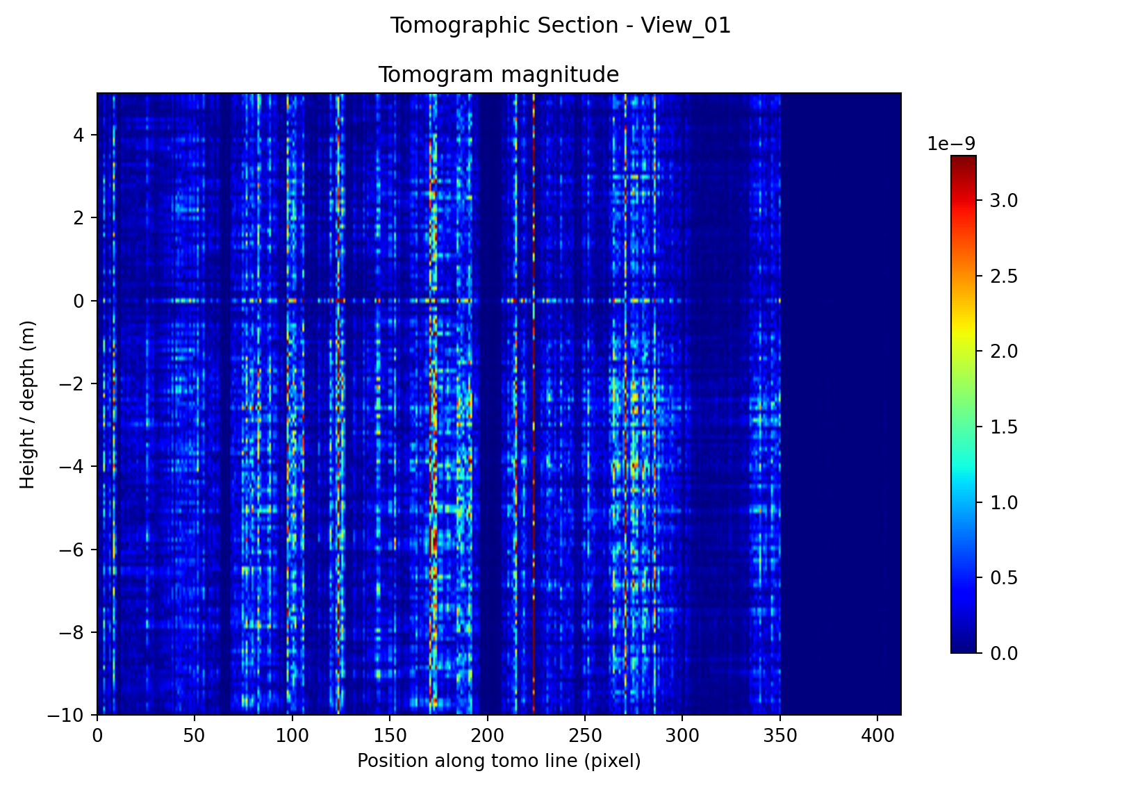
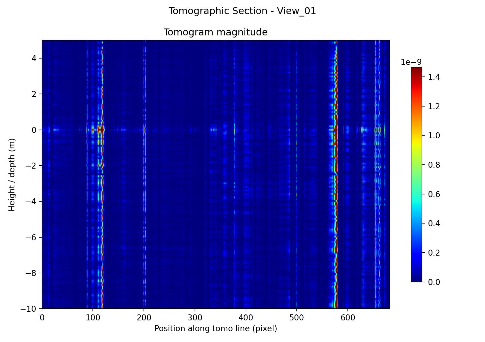
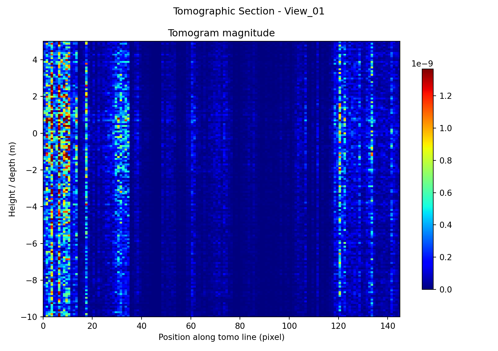
Figure 2 shows that the method does not collapse to a visually random or uniform output across all sites. Instead, each test case produces a distinct spatial pattern along the tomographic line. A common characteristic of all three reconstructions is that the dominant response is largely columnar: strong returns are concentrated at particular positions along the line and extend through a substantial portion of the plotted depth axis. This means that, at the present parameter settings, the reconstructions are better interpreted as highlighting position-dependent coherent response than as sharply resolved compact depth reflectors. Even so, the results are qualitatively meaningful because low-response regions remain dark, bright features occur at stable positions, and the structure of the sections varies in a way that is consistent with the very different physical character of the three targets. Because each panel is displayed with its own color scale, the comparison is based on the location and organization of features rather than on the absolute displayed intensity.

Bull Wall Bridge.

The bridge section exhibits a comparatively distributed response, with multiple bands of elevated magnitude appearing over broad portions of the line rather than collapsing into a single isolated scatterer. That behaviour is plausible for a slender timber bridge composed of repeated structural members, joints, decking, and supports, where several nearby elements may contribute coherently to the reconstructed signal. The section also contains a visibly dark zone toward one end of the line, which is consistent with either weaker illumination, reduced coherence, or a portion of the profile that does not intersect a strongly responding structural element. Overall, the bridge result is qualitatively credible as an elongated structural target with several active response locations rather than one dominant point-like source.

Promenade Road.

The road section is notably sparser than the bridge case. Its energy is concentrated into a small number of narrow, high-magnitude columns separated by large low-response intervals. This is consistent with the expectation that a road corridor on made ground is a weaker and less spatially coherent tomography target: the dominant contributors are more likely to be isolated bright scatterers such as edges, barriers, roadside fixtures, or transient traffic-related responses than a continuous mechanically stiff structure. The absence of a broad, continuous depth-focused signature therefore does not contradict the target hypothesis; instead, it supports the interpretation of Promenade Road as a plausible but comparatively weak test case.

Poolbeg Generating Station.

The Poolbeg section shows concentrated high-response regions at specific positions along the line, together with weaker intermediate structure. Compared with the road case, the response appears more persistently organized and more strongly tied to a small number of dominant locations, which is consistent with a radar-bright industrial site containing large metallic structures and potential machinery-related excitation sources. At the same time, the result is still dominated by vertically extended streaks rather than compact depth-localized peaks, so the image should be interpreted cautiously: it supports the presence of coherent target-dependent response, but it does not by itself prove detailed internal structural resolution.

Taken together, these three examples provide a useful first-pass validation of the pipeline. The outputs are target-dependent, spatially structured, and free of obvious gross failures such as global corruption, complete decorrelation, axis inversion, or uniform artifact filling. This is the main purpose of the qualitative validation stage in the present report: to show that the implemented workflow can ingest a real TerraSAR-X SSC scene, follow the selected tomographic line, and produce interpretable tomographic sections whose behaviour changes sensibly from one site to another.

When the same inversion is executed with the optimized backends, the expected qualitative content is preserved. In visual terms, the accelerated variants should reproduce the same section geometry and the same dominant response locations as the serial baseline, because they differ only in execution backend rather than in the mathematical formulation of the inversion. In particular, qualitative inspection should confirm that the optimized variants preserve:

• tomographic section shape: no visible shifts, flips, stretching, or truncation of the reconstructed section relative to the serial baseline;
• dominant peaks: between runs, the strongest response columns occur at the same positions along the tomographic line and retain the same broad organization over depth;
• phase / magnitude consistency: any differences are limited to small floating-point-level variation and do not produce visibly different amplitude patterns or phase-related artifacts;
• qualitative interpretation: the bridge remains the more distributed structural case, the road remains the sparsest and weakest case, and the generating station remains the most clearly localized industrial target.

Accordingly, the qualitative validation supports two conclusions. First, the overall pipeline is operational and produces physically plausible tomographic sections on real data. Second, the OpenMP and CUDA implementations can be treated as faithful computational accelerations of the same underlying reconstruction, not as altered methods that change the visual interpretation of the result.

The benchmark matrix contains three repeated runs per configuration. To reduce sensitivity to run-to-run jitter, all single-case values reported below use the median of those repeats. The repeatability of the timings was generally good: for most cells the coefficient of variation was approximately \(1.5%\), so the backend ordering is stable and not driven by isolated outliers.

Because the available measurements record runtime but not peak host/device memory, the comparison in this section is restricted to execution time. Rather than back-filling unsupported RAM or VRAM numbers, the table reports only quantities that are directly measured by the benchmark matrix.

Backend	Aggregate time [s]	Aggregate time [h]	Speedup vs.\ serial
Serial CPU	21424.4	5.95	1.00
OpenMP CPU	8034.2	2.23	2.67
CUDA	5353.6	1.49	4.00

The performance ordering is unambiguous. Over the common benchmark subset, OpenMP reduces the total runtime from \(5.95\) h to \(2.23\) h, while CUDA reduces it further to \(1.49\) h. In other words, the OpenMP backend provides a \(2.67\times\) acceleration over the serial CPU baseline, and the CUDA backend provides a \(4.00\times\) acceleration. These gains are substantial enough to change the practical usability of the workflow: the full sweep that would occupy most of a working day on the serial baseline is reduced to a few hours on the optimized backends.

The speedup is also remarkably consistent across sites and problem sizes. For example, at the bridge site with the largest recorded case, the median runtimes are \(10432.4\) s (serial CPU), \(3912.1\) s (OpenMP), and \(2608.1\) s (CUDA), preserving essentially the same ordering and almost the same multiplicative gains seen in the aggregate totals. This stability indicates that the backend changes act primarily on execution efficiency, not on the numerical behaviour of the reconstruction itself.

Taken together, the timing results support two conclusions. First, shared-memory parallelism already delivers a strong practical improvement, so the inversion is well matched to CPU-side parallel execution over independent tomographic-line pixels. Second, the CUDA implementation produces the best overall runtime, showing that the repeated dense linear-algebra work of the inversion is also a good fit for GPU batching.

The benchmark matrix most strongly supports scalability analysis with respect to the recorded size parameter \(N_{\text{sub}}\), which is the dominant variable swept in the timing runs. The matrix also includes three different line lengths (\(L=145\), \(412\), and \(682\) pixels), but these are coupled to different physical sites and scene-dependent settings, so they provide only a partial proxy for pure line-length scaling. By contrast, no controlled sweep over pair count \(P\), OpenMP thread count, or CUDA batch size was present in the recorded results, so those factors cannot be quantified here without over-interpreting the data.

Scaling with \(N_{\text{sub}}\).

The clearest trend in the matrix is the growth with \(N_{\text{sub}}\). For the bridge and substation cases, doubling \(N_{\text{sub}}\) from \(32\rightarrow64\rightarrow128\rightarrow256 \rightarrow512\) increases runtime by roughly a factor of two at each step on all three backends (about \(1.92\times\) to \(1.98\times\) per doubling). Over that range, the dominant scaling is therefore close to linear in \(N_{\text{sub}}\). The backend curves in Figure 4 are nearly parallel, which means that OpenMP and CUDA reduce the constant factor of the computation without materially changing its observed growth law.

At the largest tested size, the increase from \(512\) to \(1024\) is steeper than the preceding doublings. On the CPU and OpenMP backends the final step is approximately \(2.29\times\) to \(2.77\times\), and the available CUDA timings show a similar upward bend. This suggests that the largest case is beginning to expose additional overheads—for example larger workspaces, less favourable cache behaviour, or solver/batching effects—beyond the near-linear regime observed at smaller sizes.

A single anomaly should also be noted explicitly: at the Quay/promenade-road site, the \(N_{\text{sub}}=512\) point is unexpectedly faster than the \(N_{\text{sub}}=256\) point in all three backends.

Scaling with line length \(L\).

The three sites correspond to line lengths of \(145\), \(412\), and \(682\) pixels, but the present matrix does not isolate \(L\) as an independent variable. In particular, the shortest line (substation, \(145\) pixels) is not always the cheapest case: at \(N_{\text{sub}}=256\), its median runtime exceeds that of both the \(412\)-pixel bridge line and the \(682\)-pixel quay line on all three backends. This shows that scene-dependent constants and other per-case effects are still large enough that the current results should not be used to fit a clean \(T(L)\) law. The matrix does, however, show that backend speedups are preserved across all three line lengths, which is the main practically relevant conclusion for the present study.

Overall, the scalability results indicate that the dominant observed cost grows approximately linearly with \(N_{\text{sub}}\) over most of the tested range, while OpenMP and CUDA preserve that trend and mainly reduce its prefactor. The current benchmark matrix is therefore sufficient to support a strong statement about backend acceleration and size scaling in \(N_{\text{sub}}\), but it is not yet sufficient for equally strong claims about isolated scaling in \(L\), \(P\), thread count, or batch size.

The present implementation supports a useful distinction between three layers: the method that is directly implied by the Biondi--Malanga papers, the engineering work required to make that method executable on real TerraSAR-X SSC data [1, 5, 6], and the later optimizations introduced to make the execution practical at useful problem sizes.

At the method level, the papers clearly imply the following chain: start from a focused SLC, form Doppler sub-apertures, compare sub-apertures to estimate micro-motion or phase-consistent displacements, organize those observations along a selected tomographic line, and reconstruct a depth-dependent response through a steering-matrix-based focusing operator [4, 3]. The use of explicit geometry terms such as \(K_z\), and the interpretation of the final stage as a Fourier-like or pulse-compression-style focusing operation, are likewise part of the published method rather than a software invention [4, 46, 7]. In that sense, the core signal model and the ordering of the main computational stages are reproduced faithfully.

What the papers do not provide is a complete software specification. They do not define a machine-checkable SSC parser, a complete metadata normalization strategy, a canonical range/azimuth axis convention, a defensive validation layer for malformed products, or a fully specified ground-to-SLC reprojection procedure for reusing the same physical line across scenes [1, 5, 6]. Those are not conceptual departures from the method; they are implementation necessities that arise when a paper workflow is translated into production-like research software.

A further class of choices is explicitly performance-driven. OpenMP worksharing, thread-local dense workspaces, CUDA batching, pinned host staging, and FFT-friendly size adjustments [42, 36, 21] do not alter the forward model \(Y=A\,h\) or the intended inverse map. They change how that map is evaluated, not what is being evaluated. The results section shows that these choices materially reduce runtime while leaving the qualitative output unchanged, which supports treating them as faithful accelerations of the same reconstruction rather than as alternative scientific methods.

A related clarification concerns the benchmark scope. The compared backends isolate the tomographic inversion backend inside an otherwise fixed scene-processing pipeline. This is an appropriate experimental design for studying inversion cost, but it also means that the reported baseline is not a fully CPU-native end-to-end implementation of the entire workflow. The paper-level claim that can be supported here is therefore narrower and more precise: the inverse problem implied by the Doppler-tomography method can be executed more efficiently with shared-memory and GPU parallelism without changing its qualitative output.

The engineering choices have consequences at five levels: fidelity, robustness, computational cost, maintainability, and extensibility.

With respect to fidelity, the most important design success is that the code keeps the method-facing objects explicit. The observation vector, the per-pixel \(K_z\) term, the steering matrix, and the depth grid remain visible entities in the implementation rather than disappearing into opaque library calls. That makes it possible to state clearly which parts are paper-faithful and which are added for execution convenience. This is especially important in reproduction work, where software pragmatism can otherwise be mistaken for a scientific claim.

With respect to robustness, several non-literal additions are justified by the realities of real SAR products [1, 6]. Canonicalization prevents silent range/azimuth transposition errors; input validation prevents geometry-dependent failures from being discovered too late; and optional confidence gating reduces the influence of weak or ambiguous motion estimates [34, 32]. These choices do not strengthen the scientific claim of the original method by themselves, but they substantially strengthen the claim that the software executes the intended method in a controlled and repeatable way.

The computational implications are equally significant. The complexity analysis shows that the front end is dominated by scene-scale FFT work and pairwise motion estimation [21, 34], while the inversion cost is dominated by repeated dense pixel-local problems with asymptotic cost

The line-based design is therefore a major engineering choice in its own right: it avoids the memory and runtime burden of reconstructing a full \(R\times C\times N_z\) cube and concentrates cost on the physically selected profile. In practice, this is one of the main reasons the method becomes tractable on workstation hardware. The observed near-linear growth with the benchmark size parameter \(N_{\text{sub}}\) is consistent with that analysis: backend optimization changes the prefactor of the computation much more strongly than its empirical growth law.

Memory behavior is similarly shaped by engineering choices. The line-first inversion keeps the final outputs at \(\mathcal{O}(LN_z)\), but the pipeline still carries scene-scale FFT and SLC buffers at \(\mathcal{O}(RC)\), plus observation and geometry arrays at \(\mathcal{O}(LP)\). OpenMP improves runtime partly by replicating workspaces per thread [42], while CUDA improves runtime partly by allocating batched steering, Gram, solve, and staging buffers [36]. The implementation is therefore not "faster for free": some of the speedup is purchased by additional temporary memory and greater resource-management complexity.

Maintainability and extensibility are affected in opposite ways. The serial inversion path is the clearest reference implementation and remains the easiest place to reason about correctness. The parallel backends, by contrast, are more difficult to debug because they introduce backend-specific solver behavior, workspace management, and failure modes. However, the same decomposition that makes the code more complex also makes it more extensible: once the forward model, geometry evaluation, and inversion backend are cleanly separated, it becomes much easier to swap damping strategies, change pair schedules, introduce alternative solvers, or move additional stages onto the GPU without rewriting the entire pipeline.

Complexity and practical suitability.

An important practical conclusion is that the method is not limited primarily by any single "tomography" formula, but by the interaction of several scaling terms [46]. Increasing the number of pairs \(P\) or the number of depth bins \(N_z\) affects every pixel-local inversion; increasing line length \(L\) multiplies that cost across the profile; and increasing sub-aperture count increases the front-end work and often the effective pair count as well. This means that the method is usable in practice only when the inversion domain is constrained sensibly. The line-based restriction is therefore not just a convenient interface choice; it is a computational strategy that makes the difference between a manageable research workflow and an impractically large 3-D reconstruction.

Scene entropy and target suitability.

Scene entropy is also important, even though it does not appear as an explicit symbol in the asymptotic formulas. Here it is best understood informally as the degree to which the scene response along the tomographic line is spatially heterogeneous, weakly coherent, or dominated by many competing scatterers rather than by a few stable ones. In that sense, the three test sites occupy different positions. Poolbeg has comparatively low effective entropy in the reconstruction: a small number of persistent, radar-bright industrial locations dominate the section, which helps interpretability even when the response is vertically extended. The bridge case has moderate entropy: the response is more distributed because multiple structural members and joints likely contribute, but it still remains organized and target-like. Promenade Road appears to have the highest nuisance entropy and the lowest coherent structural concentration: energy is sparse, intermittent, and more consistent with isolated scatterers or transient excitations than with a single stiff vibrating object.

This matters because scene entropy affects the method in ways that asymptotic complexity alone does not capture. A low-entropy, strongly coherent scene tends to yield cleaner motion estimates and a more stable qualitative interpretation. A high-entropy or weakly coherent scene can produce noisier pairwise measurements, more ambiguous columns in the tomogram, and a greater dependence on gating, regularization, or interpretive caution [34, 32, 46]. The computational cost may remain nominally the same, but the value of that computation changes: the same number of floating-point operations can produce either an interpretable section or an ambiguous one depending on target structure, source stability, and coherence.

A strictly literal reading of the papers would encourage applying the stated steering-matrix inversion as directly as possible. In software, however, literalness and robustness are not always aligned. Small dense systems can become ill-conditioned when the local observation geometry is weak, when \(K_z\) samples cluster unfavorably, or when the scene provides only weak and noisy pairwise measurements [25, 7, 46]. In those cases, a software path that insists on an undamped pseudoinverse may be closer to the printed formula but farther from a stable and interpretable reconstruction.

For that reason, regularization and fallback paths should be understood as deliberate non-literalities introduced to protect the computation from numerical failure. Diagonal loading or a Tikhonov-like damped solve changes the inverse operator, but often in a controlled and transparent way: it trades some idealized resolution for reduced sensitivity to noise and near-singularity [25]. Likewise, a Cholesky-first / LU-fallback strategy in CUDA is not a change in scientific objective; it is a numerical strategy for ensuring that the same inverse problem can still be solved when the more specialized factorization path is not appropriate for a given local matrix [31, 30].

The same logic applies to confidence gating and optional signal conditioning. Thresholding on NCC quality or cross-magnitude can improve practical behavior by preventing clearly untrustworthy motion estimates from contributing to the tomogram [34, 32]. Optional bandpass filtering or envelope products can make downstream interpretation easier. But these operations also move the workflow away from a strictly literal, paper-minimal implementation, because they encode additional assumptions about which observations should count as trustworthy and which parts of the signal are of greatest interest.

The results suggest that these robustness-oriented choices are worth separating explicitly rather than hiding. The qualitative sections are already dominated by vertically extended columns rather than sharply localized compact reflectors. That is a sign that the inversion is operating in a regime where conditioning, coherence, and model mismatch matter at least as much as nominal algebra [25, 46]. In such a regime, pretending that a heavily engineered solver is still an "exact" realization of \(A^\dagger y\) would be less honest than stating directly that practical reconstruction quality depends on controlled departures from the most literal implementation.

The best compromise is therefore not maximal literalness, but switchable literalness. A useful reproduction-oriented software design should allow a near-paper mode in which optional gating, conditioning, and damping are disabled or minimized, while also supporting a robust mode for routine use on real scenes. That separation preserves methodological clarity: one can report which results are closest to the published derivation and which results rely on additional numerical safeguards.

Several limitations remain, and they should qualify both the methodological and the performance claims of this report.

First, the implementation still inherits a fundamental limitation of the underlying method: it is not conventional multi-pass TomoSAR with an externally synthesized elevation aperture, but a single-SLC Doppler-diversity construction [46, 4, 3]. As a result, the reconstructed sections should be read primarily as depth-parameterized coherent response maps, not automatically as uniquely resolved internal structure. The vertically extended, columnar character of the qualitative results makes this caution especially important.

Second, the method remains strongly dependent on metadata quality and geometry consistency. Per-pixel \(K_z\) values, line reprojection, and the final focusing operator all depend on correct timing, orbit, and geolocation support data [1, 6, 7]. Errors or inconsistencies in those inputs can produce quietly biased reconstructions even when the code itself is functioning correctly. This dependence is particularly important when the same physical line is reused across scenes through reprojection.

Third, computational scaling remains a real practical constraint. Even with the line-based design, the inversion cost still grows with \(L\), \(P\), and \(N_z\), and the memory footprint still contains scene-scale \(\mathcal{O}(RC)\) terms plus line-scale \(\mathcal{O}(LP)\) and \(\mathcal{O}(LN_z)\) terms. Large pair counts, dense depth grids, or aggressive diagnostic saving can therefore make the workflow memory-bound before it becomes mathematically interesting. The largest benchmark points already suggest that overheads begin to increase beyond the near-linear regime seen at smaller sizes.

Fourth, the present optimized implementations improve usability at the cost of software complexity. The CUDA backend in particular depends on batching strategy, device memory staging, solver library behavior, and backend-specific fallback logic [36, 31, 30]. That makes the code harder to audit and more difficult to reproduce exactly across toolchain versions and hardware generations than the serial reference path.

Fifth, the present performance study is narrower than a full-system portability study. The compared configurations isolate the inversion backend inside a fixed overall pipeline, so the reported gains should be interpreted as gains for the tomographic inversion stage and the end-to-end workflow built around it, not as a universal statement about every possible implementation of the method.

Finally, the timing dataset itself should be read with caution. Because of time constraints, part of the Serial-CPU and OpenMP performance data used for comparison were estimated from the available CUDA timings together with the known algorithmic structure, batching policy, and test setup on the same workstation, rather than obtained through a complete independent direct measurement campaign. Those values are therefore useful as engineering estimates of relative backend cost, but they are not as strong as a fully measured benchmark matrix and should not be over-interpreted as definitive hardware-level performance characterizations.

Taken together, these limitations do not invalidate the main conclusions of the report, but they do set their scope. The present study shows that the Biondi--Malanga workflow can be mapped into a working software pipeline, that this mapping requires explicit engineering decisions beyond the papers, and that parallel backends materially improve feasibility [4, 3, 42, 36]. What it does not yet show is that every reconstructed bright column has a unique physical interpretation, or that the present benchmark matrix exhausts the performance behavior of the method across all platforms and parameter regimes.

This report set out to determine whether the Doppler-domain tomography workflow described by Biondi and Malanga can be turned into working research software, which additions are required to make it executable on real TerraSAR-X SSC products, and how much practical benefit is obtained from parallel execution. The main conclusion is that the method can be reproduced faithfully at the level of its core signal model—focused SLC input, Doppler sub-aperture synthesis, inter-sub-aperture motion estimation, per-pixel \(K_z\) evaluation, and steering-matrix-based tomographic focusing—but only after adding a substantial implementation layer that is not specified in the papers themselves [3, 4, 1, 5, 6]. The qualitative results and backend comparisons further show that these additions preserve the intended reconstruction while making the workflow robust enough to run repeatedly on real scenes and fast enough to support comparative experiments (Table 4, Figure 4).

At the methodological level, the implementation supports a clear paper-to-code reconstruction. The published workflow starts from a focused SLC, partitions the azimuth spectrum into Doppler sub-apertures, estimates relative motion between sub-aperture looks, and reconstructs a depth-dependent response by applying a steering-matrix-based inverse model along a selected tomographic line [3, 4]. Those same objects remain explicit in the software: the observation vector, the per-pixel \(K_z\) term, the depth grid, and the final inversion operator are all represented directly rather than hidden inside a black-box processing chain. That is the strongest sense in which the implementation is faithful to the reference method: it preserves not only the broad order of operations, but also the mathematical entities that carry the scientific meaning of the reconstruction [3, 4, 46, 7].

The line-based design is particularly important. In the present implementation the inversion is restricted to a user-defined tomographic profile, which is consistent with the way the reference workflow computes a tomogram along a contiguous line of pixels rather than requiring a full scene-wide voxel reconstruction [3]. This choice preserves the intended signal-processing logic while making the computation substantially more manageable than a full \(R\times C\times N_z\) volume, a distinction that is also important in the broader TomoSAR literature, where volumetric reconstruction is well known to increase both computational and memory costs [9, 46].

A second conclusion is that literal reproduction of the papers is not sufficient for a reliable software implementation. Real TerraSAR-X SSC products require product parsing, metadata extraction, axis canonicalization, and geometry normalization before the published inversion model can even be applied consistently [1, 5, 6]. Likewise, reusing the same physical tomographic line across scenes requires a ground-to-SLC reprojection step that is operationally necessary even though it is not written as a complete software recipe in the reference papers [1, 6].

The same is true on the numerical side. Sub-aperture comparison and offset estimation benefit from well-established registration practice such as normalized cross-correlation, phase-correlation ideas, and sub-pixel interpolation, especially when observations are noisy or weakly textured [29, 33, 45, 2]. Confidence gating and stacking-oriented robustness measures are likewise defensible engineering additions when pairwise motion estimates are uneven in quality [34, 32]. Finally, regularization and fallback solves are justified because small tomographic systems can become ill-conditioned when the effective sampling geometry is weak or when the measurements are noisy; in that regime, Tikhonov-style damping and stability-oriented solver choices are standard tools for controlling sensitivity to perturbations [25, 26, 46, 7]. These additions are therefore best understood not as changes to the scientific goal, but as the minimum engineering needed to execute the intended inverse problem robustly on real data.

The results of the implementation study show that the dominant computational burden is shaped by the interaction of scene-scale FFT work, pairwise motion estimation, and repeated pixel-local tomographic inversions. That pattern is consistent with the computational structure of FFT-based signal processing and dense linear-algebra-based inverse problems more generally [21, 46, 25]. The most consequential engineering choice for tractability is therefore the line-first inversion design: the output scales as \(L\times N_z\) rather than \(R\times C\times N_z\), while the unavoidable scene-scale terms are largely confined to SLC preparation and sub-aperture synthesis. In practice, this is the choice that most strongly controls memory growth and keeps the workflow feasible on workstation hardware [9, 46].

The optimization study shows that the inversion stage is also structurally well suited to parallelism. OpenMP maps naturally onto independent per-pixel inversion work in shared memory, whereas CUDA is well matched to batched dense algebra and repeated accelerator-resident kernels [42, 36, 31, 30]. The measured results confirm that this structural match matters in practice: over the common benchmark subset, OpenMP reduces aggregate runtime from \(5.95\) h to \(2.23\) h, and CUDA reduces it further to \(1.49\) h (Table 4). That corresponds to measured speedups of \(2.67\times\) for OpenMP and \(4.00\times\) for CUDA relative to the serial CPU baseline. Moreover, the runtime curves remain close to linear in \(N_{\text{sub}}\) over most of the tested range (Figure 4), indicating that the optimized backends mainly reduce the prefactor of the computation rather than changing its empirical growth law. The practical consequence is straightforward: what is close to a full-day sweep in the serial baseline becomes a workflow that is much easier to iterate, benchmark, and debug on accelerated backends.

Taken together, the study supports four final claims. First, the Biondi--Malanga Doppler tomography workflow is implementable as a coherent and reproducible software pipeline when the method-facing quantities are kept explicit and the input geometry is handled carefully [3, 4, 1]. Second, a substantial fraction of the work needed for a usable implementation lies outside the papers themselves and takes the form of software engineering, numerical stabilization, and data-handling decisions rather than new scientific modeling [6, 34, 25]. Third, the choices that matter most for complexity and memory are the restriction to a tomographic line, the management of scene-scale FFT buffers, and the replication or batching of dense inversion workspaces for OpenMP and CUDA execution [21, 42, 36]. Fourth, OpenMP and CUDA materially improve the practical feasibility of the method without changing its qualitative output, so they are best viewed as faithful accelerations of the same inversion rather than as distinct reconstruction methods.

At the same time, the limits identified in the discussion remain important. Because this is a single-SLC Doppler-diversity construction rather than a conventional multi-pass elevation aperture, the reconstructed sections should be interpreted primarily as depth-parameterized coherent response maps, not as automatically unique internal-structure solutions [3, 4, 46, 9]. Future work should therefore focus not only on faster execution, but also on stronger uncertainty characterization, controlled sweeps over \(L\), \(P\), and \(N_z\), and more systematic comparison between near-paper and robust execution modes. Even with those caveats, the present report establishes its central point: the method is scientifically reproducible in software, computationally nontrivial, and substantially more usable once the inversion is engineered and accelerated with explicit attention to robustness, memory, and backend-aware parallelism.

Promenade Rd. [-6.1894024, 53.3502275] to [-6.1964215, 53.3502805]

Dollymount Wooden Bridge. [-6.1798645, 53.3597082] to [-6.1811655, 53.3601985]

Poolbeg Generating Station. [-6.1886728, 53.3395279] to [-6.1901730, 53.3395891]

Data ingestion and metadata extraction.

The pipeline begins with conversion of the raw TerraSAR-X / TanDEM-X SSC product into an internal single-look complex (SLC) representation. During this stage, the software extracts the metadata required for downstream processing, including raster dimensions, acquisition parameters, orbit-related information, and geolocation support data. The result is a standardized scene package that can be consumed uniformly by the runtime.

Scene / view discovery.

Once the input has been prepared, the runtime scans the provided directory structure and identifies all valid scenes or views available for processing. Each discovered scene is checked for the expected SLC and metadata products, and the resulting collection defines the set of acquisitions that participate in the current tomographic run.

Tomographic line definition.

The tomographic reconstruction is not performed over the full image but along a selected line or profile. This line may be specified directly in image coordinates or through ground-referenced coordinates that are reprojected into the SAR scene. This design allows the software to focus computation on the physically relevant cross-section while also supporting consistent alignment across multiple scenes.

Preprocessing and canonicalization.

Before heavy computation begins, each scene is validated and transformed into a canonical internal representation. This includes enforcing a consistent range--azimuth axis convention, normalizing metadata layout, and expressing the tomographic line coordinates in the same internal reference frame. By standardizing the scene representation at this stage, later modules can operate without repeated format-dependent branching.

GPU front-end processing.

The front-end stage performs the main signal-processing operations required to generate tomographic observations. These operations include Doppler sub-aperture formation, construction of master/slave pair schedules, local coregistration, and cross-spectral or motion-related measurement extraction. The computationally intensive image-domain processing is executed on the GPU so that large numbers of sub-aperture and pairwise operations can be handled efficiently.

Tomographic inversion backend.

The measurements produced by the front end are then combined with the scene geometry model, particularly the per-pixel \(K_z\) values, to recover the tomographic section along the selected height axis. The software supports multiple inversion backends, including a baseline CPU path, an OpenMP-parallel CPU path, and a CUDA-based implementation. Each pixel along the tomographic line is inverted independently, making the approach naturally amenable to parallel execution.

Output writing and diagnostics.

After inversion, the software writes the reconstructed tomographic magnitude and phase products together with the corresponding geometry descriptors, schedules, intermediate observations, and execution diagnostics. This output design makes the pipeline suitable not only for reconstruction but also for debugging, validation, reproducibility, and performance analysis, since important intermediate products are preserved alongside the final result.

Notes

1. See appendix B for a pipeline overview.
2. See appendix A for exact tomo-line coordinates.

References

1. {Airbus Defence and Space}. TerraSAR-X Image Product Guide: Basic and Enhanced Radar Satellite Imagery, 2014. Issue 2.0, August 2014.
2. Alfonso Alba, Ruth M. Aguilar-Ponce, Javier Flavio Vigueras-G{omez, and Edgar Arce-Santana. Phase correlation based image alignment with subpixel accuracy. In Advances in Artificial Intelligence, volume 7629 of Lecture Notes in Computer Science, pages 171--182. Springer, Berlin, Heidelberg, 2013. MICAI 2012.
3. Filippo Biondi. Scanning inside volcanoes with synthetic aperture radar echography tomographic doppler imaging. Remote Sensing, 14(15):3828, 2022.
4. Filippo Biondi and Corrado Malanga. Synthetic aperture radar doppler tomography reveals details of undiscovered high-resolution internal structure of the great pyramid of giza. Remote Sensing, 14(20):5231, 2022.
5. Helko Breit, Birgit Sch{attler, Thomas Fritz, Ulrich Balss, Heiko Damerow, and Egbert Schwarz. Terrasar-x payload data processing: Results from commissioning and early operational phase. In Proceedings of the IEEE International Geoscience and Remote Sensing Symposium (IGARSS), pages II--209--II--212, 2008.
6. Stefan Buckreuss, Birgit Sch{attler, Thomas Fritz, Josef Mittermayer, Ralph Kahle, Edith Maurer, Johannes B{oer, Markus Bachmann, Falk Mrowka, Egbert Schwarz, Helko Breit, and Ulrich Steinbrecher. Ten years of terrasar-x operations. Remote Sensing, 10(6):873, 2018.
7. Victor Cazcarra-Bes, Matteo Pardini, and Kostas Papathanassiou. Definition of tomographic sar configurations for forest structure applications at l-band. IEEE Geoscience and Remote Sensing Letters, 19:1--5, 2022.
8. Ulrike Dackermann, Keith Crews, Bohumil Kasal, Jianchun Li, Mariapaola Riggio, Frank Rinn, and Thomas Tannert. In situ assessment of structural timber using stress-wave measurements. Materials and Structures, 47:787--803, 2014.
9. Gustavo Daniel Mart{\'\i}n del Campo-Becerra, Andreas Reigber, Matteo Nannini, and Scott Hensley. Single-look {SAR} tomography of urban areas. Remote Sensing, 12(16):2555, 2020.
10. Ricardo Dobry, Tarek H. Abdoun, K. H. Stokoe II, Richard E. S. Moss, Michael Hatton, and Hesham El Ganainy. Liquefaction potential of recent fills versus natural sands located in high-seismicity regions using shear-wave velocity. Journal of Geotechnical and Geoenvironmental Engineering, 141(3):04014112, 2015.
11. {DORIS Development Team}. Baseline. https://doris.tudelft.nl/usermanual/node182.html, 2008. DORIS user manual page, accessed: 2026-03-14.
12. {Dublin City Council}. North bull island. https://www.dublincity.ie/parks-and-nature/dublin-city-parks/visit-park/north-bull-island. Accessed: 2026-03-14.
13. {Dublin Port Company}. Masterplan: Issues paper. https://www.dublinport.ie/wp-content/uploads/2017/01/Issues_Paper.pdf, 2011.
14. {Dublin Port Company}. Promenade road extension opening -- 12th january 2022. https://www.dublinport.ie/promenade-road-extension-opening-12th-january-2022/, 2021. Published 22 December 2021.
15. {Dublin Port Company}. Bull island wooden bridge inspection. https://www.dublinport.ie/bull-island-wooden-bridge-inspection/, 2022. Published 5 July 2022.
16. {Dublin Port Company}. Annual report and financial statements 2023. https://www.dublinport.ie/wp-content/uploads/2024/06/DPC_Annual_Report_2023_English_FINAL.pdf, 2024.
17. {ESB}. Poolbeg -- thermal. https://esb.ie/what-we-do/generation-and-trading/poolbeg---thermal. Accessed: 2026-03-14.
18. {ESB Archives}. Poolbeg power station. https://esbarchives.ie/wp-content/uploads/2016/03/Poolbeg-Power-Station_Inventory-Book.pdf, 2023. Inventory book.
19. {European Space Agency}. {ESA Catalog -- TerraSAR-X}. https://eocat.esa.int/eo-catalogue/collections/TerraSAR-X. Accessed: 2026-03-14.
20. {Evident Scientific}. Material sound velocities. https://ims.evidentscientific.com/en/learn/ndt-tutorials/thickness-gauge/appendices-velocities. Accessed: 2026-03-14.
21. Matteo Frigo and Steven G. Johnson. FFTW 3.3.10 Manual, 2020.
22. Thomas Fritz. TerraSAR-X Ground Segment Level 1b Product Format Specification. German Aerospace Center (DLR), December 2007. Issue 1.3.
23. Thomas Fritz and Manfred Eineder. TerraSAR-X Basic Product Specification Document. German Aerospace Center (DLR), October 2013. Public version 1.9.
24. {Global Energy Monitor}. Poolbeg power station. https://www.gem.wiki/Poolbeg_power_station. Accessed: 2026-03-14.
25. Gene H. Golub, Per Christian Hansen, and Dianne P. O'Leary. Tikhonov regularization and total least squares. SIAM Journal on Matrix Analysis and Applications, 21(1):185--194, 1999.
26. Per Christian Hansen. The {L}-curve and its use in the numerical treatment of inverse problems. In P. Johnston, editor, Computational Inverse Problems in Electrocardiology, volume 4 of Advances in Computational Bioengineering, pages 119--142. WIT Press, 2000.
27. Thomas L. Holzer, Amy C. Padovani, Michael J. Bennett, Thomas E. Noce, and John C. Tinsley. Mapping {NEHRP} {VS30} site classes. Earthquake Spectra, 21(2):353--370, 2005.
28. Gang Hong. Image Fusion, Image Registration, and Radiometric Normalization for High Resolution Image Processing. PhD thesis, University of New Brunswick, Fredericton, New Brunswick, Canada, 2007. Ph.D. dissertation, Department of Geodesy and Geomatics Engineering, Technical Report No. 247.
29. Artan Kaso. Computation of the normalized cross-correlation by fast fourier transform. PLOS ONE, 13(9):e0203434, 2018.
30. {LAPACK}. Gesv: Factor and solve a general system of linear equations, 2025. Netlib LAPACK documentation.
31. {LAPACK}. Posv: Driver for solving linear systems with a hermitian/symmetric positive definite matrix, 2025. Netlib LAPACK documentation.
32. Silvan Leinss, Shiyi Li, Yajing Yan, and Bas Altena. Sar offset tracking. In Surface Displacement Measurement from Remote Sensing Images, pages 59--87. Wiley, 2022.
33. J. P. Lewis. Fast normalized cross-correlation. https://scribblethink.org/Work/nvisionInterface/nip.pdf, 1995. Expanded version of a Vision Interface 1995 paper.
34. Shiyi Li, Silvan Leinss, and Irena Hajnsek. Cross-correlation stacking for robust offset tracking using sar image time-series. IEEE Journal of Selected Topics in Applied Earth Observations and Remote Sensing, 14:4765--4778, 2021.
35. {MathWorks}. envelope -- signal envelope -- {MATLAB}. https://www.mathworks.com/help/signal/ref/envelope.html. Accessed: 2026-03-14.
36. {NVIDIA}. CUDA C++ Best Practices Guide, 2024. Release 12.5.
37. {NVIDIA Corporation}. cuBLAS, 2026. Release 13.2.
38. {NVIDIA Corporation}. {CUDA C++ Best Practices Guide}, 2026. Release 13.2.
39. {NVIDIA Corporation}. cuFFT, 2026. Release 13.2.
40. {NVIDIA Corporation}. cuSOLVER, 2026. Release 13.2.
41. {OpenMP Architecture Review Board}. {OMP_STACKSIZE}. https://www.openmp.org/spec-html/5.0/openmpse54.html. OpenMP specification page, accessed: 2026-03-14.
42. {OpenMP Architecture Review Board}. OpenMP Application Program Interface Version 4.5, November 2015.
43. {OpenMP Architecture Review Board}. OpenMP API 5.2 Reference Guide, 2021. Accessed: 2026-03-14.
44. {OpenMP Architecture Review Board}. OpenMP Application Programming Interface, 2021. Version 5.2, November 2021.
45. Luca Pallotta, Gaetano Giunta, and Carmine Clemente. Subpixel {SAR} image registration through parabolic interpolation of the {2D} cross-correlation. IEEE Transactions on Geoscience and Remote Sensing, 58(6):4132--4144, 2020.
46. Yuanyuan Wang and Xiao Xiang Zhu. Sar tomography via nonlinear blind scatterer separation. IEEE Transactions on Geoscience and Remote Sensing, 59(7):5751--5763, 2021.
47. {Weslin}. Wooden bridge, bull island. https://weslin.ie/weslin-portfolio/wooden-bridge-bull-island/. Accessed: 2026-03-14.
48. Peter Wood. Promenade road at the port of dublin. https://www.geograph.ie/photo/5588098. Geograph Ireland, accessed: 2026-03-14.