Abstract

We treat seasonal-to-interannual forecasting of tropical-Pacific sea-surface temperature (SST) as a multiscale field-forecasting problem. Two 14-month products are built on a $24\times48$ tropical-Pacific grid from ERA5 monthly SST (1981–2025), operate in an exactly invertible 37-channel dual-tree complex-wavelet space, and predict relative SST anomalies (departures from a causal 30-year trailing climatology with the tropical-Pacific mean removed): a deterministic persistence-residual Earthformer, pretrained on CMIP6 simulations and fine-tuned on 1981–2020 observations, and a 32-member ensemble sampled once from a temporally joint residual-diffusion head around the frozen deterministic center. On 47 overlapping validation windows with 2021–2025 targets—a development period also used for checkpoint selection, so no untouched test period exists—the deterministic model beats anomaly persistence at all 14 leads (field RMSE $0.622$ versus $0.779\,{}^{\circ}\mathrm{C}$), and an ablation shows the CMIP6 pretraining is necessary for that skill. A 20-mode linear inverse model, however, attains lower field RMSE ($0.559\,{}^{\circ}\mathrm{C}$) and keeps that advantage when rescaled to the learned model's amplitude; the learned model's remaining edge is the highest long-lead Niño-3.4 correlation ($0.662$ versus $0.550$), a margin within sampling uncertainty on this record. The ensemble retains lowpass continuity, realistic amplitude, and the center's index correlation, but carries a systematic center displacement (approximately $+0.070\,{}^{\circ}\mathrm{C}$ field RMSE across ten seed replications), no detectable flow-dependent spread signal on this record, and 80/90% intervals that under-cover (66.7/71.8%) after spread-only calibration; recentering the archived deviations on the deterministic trajectory would improve fair CRPS from $0.399$ to $0.325\,{}^{\circ}\mathrm{C}$. Three predeclared product-adoption criteria are accordingly not met. The study delivers a pretraining-dependent deterministic forecast whose demonstrated value lies in long-lead index coherence rather than bulk field error, and a quantified characterization of residual diffusion around a frozen center that fixes the requirements—temporally correlated, state-dependent, mean-preserving sampling—for any successor generative head.

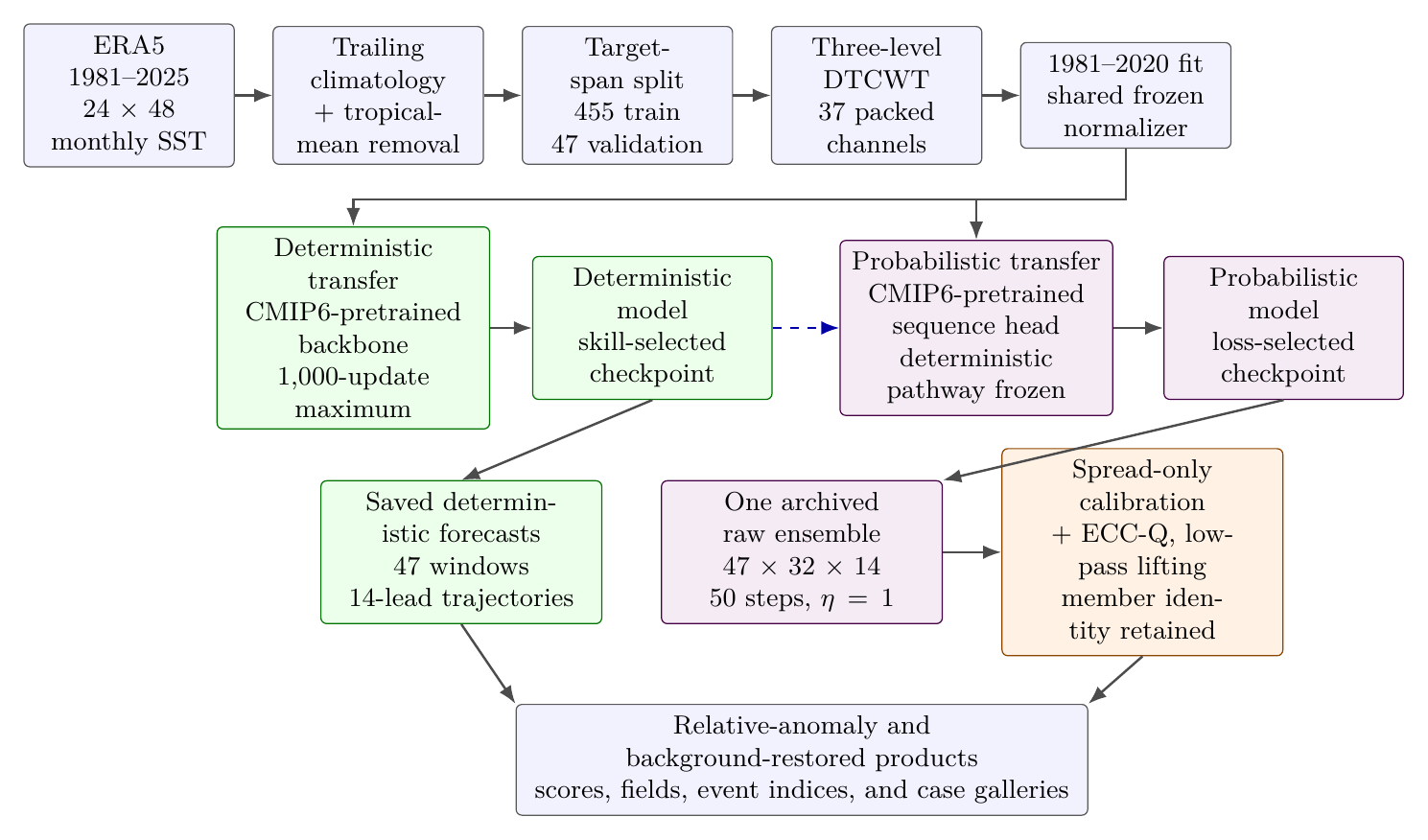
Skillful forecasts of tropical-Pacific SST at seasonal-to-interannual range underpin ENSO outlooks and their downstream users; this study asks what a modern spatiotemporal transformer, given only monthly SST, adds to that problem—and characterizes, rather than assumes, the behavior of a diffusion ensemble built on top of it. The forecast task is fixed throughout: given 12 consecutive monthly SST fields on an endpoint-inclusive $24\times48$ grid spanning $30^{\circ}$S–$30^{\circ}$N and $120^{\circ}$E–$280^{\circ}$E (grid spacing ${\approx}2.61^{\circ}$ latitude by ${\approx}3.40^{\circ}$ longitude), predict the next 14 monthly fields. Two products address this task. The deterministic model produces a single 14-month relative-SST-anomaly trajectory. The probabilistic model freezes the deterministic pathway and adds a temporally joint residual-diffusion head, from which a 32-member trajectory ensemble is sampled. The two products share the same ERA5 source, anomaly construction, coefficient normalizer, deterministic center, target dates, physical validity mask, and inverse wavelet transform.

The study makes three contributions. First, it characterizes what a coefficient-native, persistence-residual Earthformer—pretrained on CMIP6 simulations and fine-tuned on a restricted decoder boundary using 1981–2020 observations—adds over reference forecasts on a 2021–2025 development-validation period: it outperforms persistence at all 14 leads, its skill is causally dependent on the CMIP6 pretraining (an ablation without it never beats persistence), and, although damped statistical references (a linear inverse model, an EOF ridge regression) attain lower pooled RMSE—an advantage the LIM retains even when rescaled to the learned model's amplitude, since correlations are invariant to rescaling—the learned model attains the highest long-lead Niño-3.4 correlation among the single-trajectory forecasts, a margin that is not resolved on this record. Second, it specifies and executes a complete probabilistic workflow (joint sequence sampling, spread-only Gaussian calibration with rank-preserving ensemble copula coupling, coherent lowpass field lifting, and a background-restored reconstruction) around a single archived ensemble, so that every probabilistic number in this paper derives from one saved artifact. Third, it provides a quantified characterization of residual diffusion around a frozen center: what the ensemble preserves (lowpass continuity, anomaly amplitude, index coherence), what it costs (a systematic center displacement across sampling seeds), and which calibration properties are and are not attainable by spread-only postprocessing, with two predeclared sensitivity variants that isolate how much of the calibrated shortfall the center displacement explains; the accompanying temporal diagnostics localize each behavior to excess high-frequency trajectory variability, yielding design requirements for temporally structured sampling.

Two properties of the evidence should be kept in view throughout. (i) The 2021–2025 windows served both for checkpoint selection and for all reported scores, so every number in this paper is a development-validation estimate, not performance on an untouched test period (Section 5.5). (ii) The acceptance criteria referred to below were fixed in version-controlled planning documents before the production runs, but they are project-defined criteria rather than an externally registered protocol.

Product	Output	Outcome
Deterministic	One 14-month relative-SST-anomaly trajectory per window	Meets all predeclared skill, initialization, normalization, and pathway-identity criteria on development validation.
Probabilistic	One archived raw 32-member trajectory ensemble; calibrated and field-lifted derivatives	Complete artifact set; the sampled-center, flow-dependence, and calibrated-coverage adoption criteria are not met.

This study treats ENSO prediction as a multiscale field-forecasting problem rather than only a scalar-index regression problem. Convolutional ENSO forecasting established the value of learning from gridded climate fields and of augmenting the short observational record with coupled-model simulations [1]. Earthformer extends spatiotemporal field learning with cuboid attention [5]; its sequence geometry directly supports the required mapping from 12 monthly Pacific fields to 14 monthly fields without compressing the state to a handful of indices.

The coefficient representation is motivated by tropical-Pacific SST structure. The dual-tree complex wavelet transform (DTCWT) supplies approximate shift invariance, directional highpass bands, and an exact inverse [3, 4]. The system keeps the complete lowpass and highpass pyramid: the lowpass represents much of the basin-scale ENSO signal, while the oriented detail bands retain localized fronts and gradients. This yields a model-native multiscale space while preserving a closed reconstruction path to physical SST.

Simulation pretraining addresses the limited observational sample. CMIP6 provides long, physically generated SST sequences [6], and simulation-pretrained weather models demonstrate that aligned synthetic-to-real transfer can improve data-driven prediction [7]. Here the alignment is explicit: pretraining and observational fine-tuning share the Pacific grid, the 12-to-14 forecast geometry, the 37-channel coefficient packing, and the persistence-residual formulation. The observational stage then updates only the final decoder block.

The probabilistic model treats unresolved evolution as a stochastic residual around the frozen deterministic trajectory, following residual-corrective diffusion in geophysical prediction [8] and the broader use of diffusion ensembles in weather forecasting [9]. Standard denoising diffusion provides the training objective [10]; joint processing of the whole lead sequence, as in temporal diffusion models [11], is intended to preserve member trajectory identity. The probabilistic objective additionally weights the four wavelet scales equally so the numerous fine-scale coefficients do not overwhelm the index-carrying lowpass.

Postprocessing remains deliberately low dimensional because only 47 validation windows are available. A spread-only Gaussian calibration—a restricted form of ensemble model output statistics (EMOS) [12]—adjusts lead-dependent Niño-3.4 spread, and ensemble copula coupling on quantiles (ECC-Q) preserves the raw member ordering [13]. Fair CRPS corrects finite-ensemble self-distance bias [14], while proper-score principles discourage improvements that arise only from distributional hedging [15]. Finally, the causal trailing climatology follows the logic of operational 30-year base-period updates [19], and removing the tropical-mean departure follows evidence that ENSO variability is better separated from a warming tropical background in a relative-SST frame [16, 17].

ERA5 monthly-mean SST [2], updated through December 2025, covers January 1981–December 2025. Source fields are standardized to Celsius, joined across the longitude seam, ordered in the $0$–$360^{\circ}$ convention, and linearly regridded to the analysis grid. Coordinate, unit, cadence, missingness, and domain-coverage checks run before coefficient construction. Missing physical cells (land) remain identified by a validity mask and are zero-filled only at the dense DTCWT boundary; the consequences of this zero fill for coastal wavelet support are discussed in Section 7.

The anomaly reference is fixed before model training. Let $b$ denote the first year of a five-year block anchored at 1981, $m$ a calendar month, $x$ a grid cell, and $S_{y,m}(x)$ SST. The reference climatology of block $b$ is the calendar-month mean over a trailing base $\mathcal Y_b$,

where $\mathcal Y_b$ contains the years of the nominal 30-year window $[b-30,\,b-1]$ that are available in the record, provided at least 20 such years exist. Because the record begins in 1981, the earliest blocks (1981–2000) lack this minimum and instead use a fixed warm-up climatology computed over 1981–2010; the 2001 and 2006 blocks use the available 1981–2000 and 1981–2005 years; and from the 2011 block onward the full 30-year trailing base is available (the 2021–2025 validation block is referenced to 1991–2020). The base is updated only at five-year boundaries, following the cadence of operational 30-year ENSO climatology updates [19]. Two properties of this construction should be noted. First, the warm-up base extends to 2010 and is therefore not strictly causal for timestamps before 2011; it lies entirely within the 1981–2020 training partition, so no information crosses the train–validation boundary, but early training anomalies are not real-time reproducible. Second, the reference changes discontinuously at block boundaries, so a single window whose context and targets straddle a boundary (for example, context months in 2020 and targets in 2021) mixes two references; the size of this effect has not been quantified (Section 7).

Throughout this paper, relative SST anomaly means the local climatological departure after removal of its contemporaneous cosine-weighted tropical-Pacific domain mean,

where $\Omega$ is the set of valid ocean cells and $\varphi_x$ the cell latitude. This separates spatial ENSO contrast from a domain-wide tropical background [16, 17]. All primary model-space products, and the headline scores in this paper, are stated in this relative-anomaly frame; Section 4.5 defines the derivative product that restores the background term.

Windows are assigned by their full target span. A training window must place all 14 targets within January 1981–December 2020; a validation window must place all targets within January 2021–December 2025. This produces 455 training and 47 validation windows. Context months may precede the target partition, as they would when issuing a forecast at the start of that partition; no target month crosses a partition boundary.

The validation windows overlap heavily. Forty-seven monthly start dates with 14 leads yield $47\times14=658$ forecast–target pairs, but these cover only 60 unique target months (January 2021–December 2025); interior target months are verified by up to 14 different forecasts, and the verifying series at any fixed lead is strongly serially correlated. Pooled scores therefore weight mid-period months—including the 2021–2022 La Niña and 2023–2024 El Niño episodes—more heavily than boundary months, and the 658 pairs cannot be treated as independent samples when judging differences between models. Paired comparisons therefore attach uncertainty with a moving-block bootstrap over the ordered windows (Section 5.1), and even those intervals rest on effectively few independent blocks. Grouping validation windows by context-start year yields four groups of 12, 12, 12, and 11 windows (context starts in 2020–2023); these four groups form the cross-validation folds used for calibration in Section 4.3.

Each monthly relative-anomaly map is transformed independently with a three-level DTCWT using near_sym_b and qshift_b filters. One real lowpass and six oriented complex highpasses per level are packed as

Each pyramid level retains its native spatial resolution (level-$l$ highpasses are dyadically decimated relative to the $24\times48$ field). To form the dense $24\times48\times37$ model tensor, every level is placed in the top-left corner of the common grid and zero-padded on its bottom and right edges; no coefficient value is interpolated. The padding geometry is recorded per channel, a channel-aligned validity mask marks the non-padded coefficient support, and the inverse operation slices channels and crops padding, so the pack/lift/unpack cycle is bit-exact. Combined with the exact DTCWT inverse, the maximum coefficient-to-field reconstruction error over the record is $1.91\times10^{-6}\,{}^{\circ}\mathrm{C}$.

A mask-aware mean and standard deviation are fitted separately for each packed channel using 1981–2020 coefficients only. This one normalizer is frozen and shared by both models for training, inference, inverse reconstruction, and field lifting.

Figure 1 shows the single fixed construction: the shared observational path, the deterministic transfer stage, and the probabilistic sampling stage. Every downstream probabilistic artifact is derived from the one saved ensemble; calibration, lifting, scoring, and figures do not invoke the sampler again.

The deterministic model is a coefficient-native Earthformer initialized from a CMIP6 forecast-pretrained backbone; the underlying Earthformer base weights are the publicly released ICAR-ENSO checkpoint of [5], over which the CMIP6 forecast pretraining was applied. Pretraining used monthly SST (tos) from 11 CMIP6 models, with three additional models held out for checkpoint selection;¹ simulation windows were source-balanced and shared the Pacific grid, 12-to-14 forecast geometry, 37-channel packing, and persistence-residual formulation of the observational stage, and each realization was cell-wise linearly detrended before referencing to a 1900–1999 climatology [6, 7]. The backbone checkpoint was selected by held-out-simulation skill and checksum-verified before observational transfer.

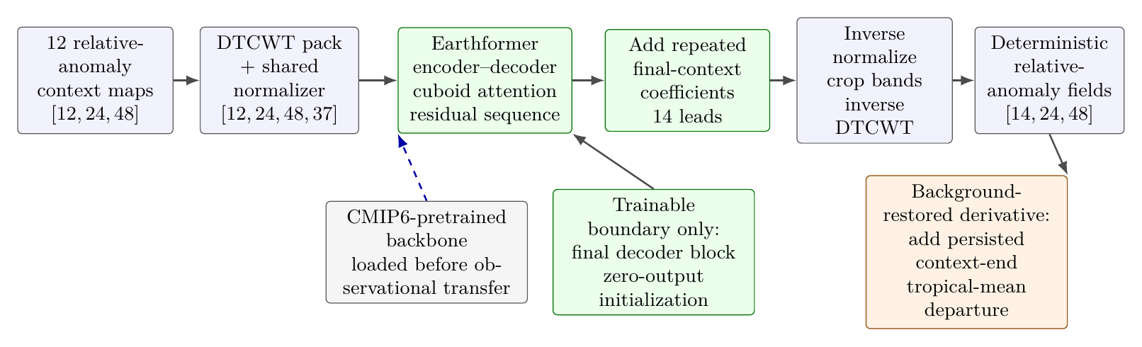
The Earthformer forecaster comprises ${\approx}1.40$ million parameters; the trainable final-decoder-block boundary comprises ${\approx}0.22$ million of them (16%), and everything else stays at its pretrained values. The observational model predicts a residual around coefficient persistence,

where $R_{\theta,\ell}$ is the Earthformer output at lead $\ell$ and $\mathcal P(a_t)$ repeats the final-context coefficients. The output projection is reset to zero before training, so the initial forecast is exactly persistence. Only the final decoder block is trainable. The training objective combines masked coefficient and reconstructed-field error, field anomaly correlation, Niño-3.4 index error, excess residual energy, and bias, with weights inherited unchanged from the simulation pretraining stage,²

Training uses AdamW (learning rate $10^{-4}$ for fresh layers, $5\times10^{-6}$ for reused layers; weight decay $10^{-5}$), batch size one, FP32, gradient clipping at 1.0, seed 42, at most four epochs with a maximum of 1,000 observational updates, and full-validation evaluation at epoch cadence and at the final update. The final checkpoint is selected by validation Niño-3.4 correlation over leads 3–14, subject to positive field anomaly correlation, field RMSE below the persistence baseline, and finite, non-collapsed variability diagnostics. The selected deterministic pathway remains bit-identical inside the probabilistic checkpoint.

The probabilistic model adds a temporally joint residual-diffusion head around the frozen deterministic center. The head is initialized from a sequence-diffusion head pretrained for 16,000 steps on the same CMIP6 corpus and selected on held-out simulation models; the deterministic pathway is frozen throughout observational training, and its tensors are verified bit-identical before and after.

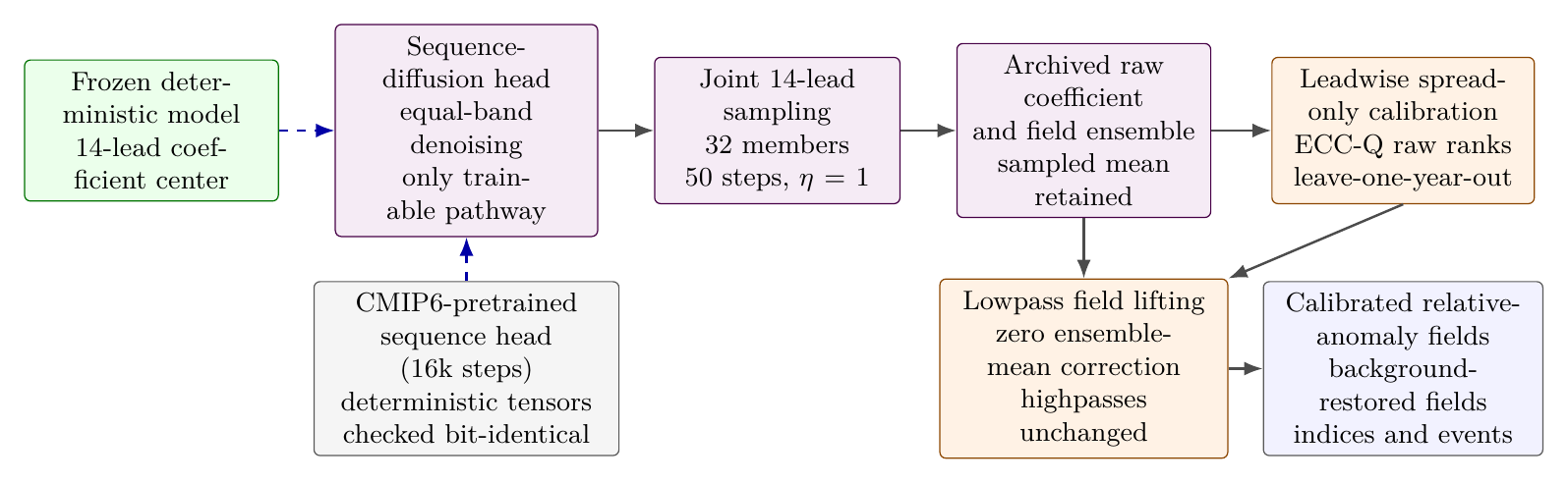
For clean residual sequence $r_0$ (the 14-lead coefficient residual around the deterministic center), diffusion time $s$, noise $\epsilon$, and wavelet band $b$, the equal-band objective is

Equal band weighting prevents the numerous fine-scale coefficients from overwhelming the lowpass. The head processes all 14 leads jointly (hidden width 32, depth 3, 1,000 diffusion timesteps, time-embedding width 64, denoised-estimate clipping at 4.0; ${\approx}1.80$ million parameters, all trainable in this stage). Only the head trains, for at most 1,000 observational updates; the checkpoint is selected by validation denoising loss, since the frozen center makes deterministic metrics invariant across candidate checkpoints.

One ensemble is generated for all 47 validation windows: 32 members, stochastic DDIM sampling with 50 steps and $\eta=1$, independent noise across leads (lead-noise correlation $\rho=0$), and metric seed 42. The finite sampled mean is retained as generated; members are not recentered on the deterministic forecast. All probabilistic scores, calibration fits, lifted fields, and figures read these saved arrays rather than sampling again. The canonical product is this single realization; to separate distributional-center bias from Monte Carlo noise, ten additional 32-member ensembles were subsequently generated from the frozen checkpoint under predeclared seeds and are reported as sensitivity evidence in Section 6.3. The canonical ensemble remains the frozen product throughout.

The Niño-3.4 index ensemble is calibrated with a spread-only Gaussian adjustment: each calibrated distribution is centered on the unchanged sampled ensemble mean $\bar q_{\ell}$, and only a lead-dependent width $\sigma_{\ell}$ is fitted [12]. The width is fitted by matching the center's error variance: a degree-2 polynomial in lead is fit to the logarithm of the per-lead mean squared difference between the verifying index and the sampled mean over the fit windows (at most three effective parameters), and $\sigma_{\ell}$ is the square root of the smoothed variance. Because the width is matched to the center's error variance, a held-out spread–skill ratio near one is largely built into the estimator; the informative calibration outcomes are the interval coverages (Section 6.4). The construction is deliberately more restrictive than conventional EMOS, which typically also permits a bias or affine mean correction; with 47 overlapping windows, the mean was left untouched to avoid refitting the center on the same period used to select it. Section 6.4 quantifies this choice with two predeclared sensitivity variants: a leave-one-year-out per-lead mean correction, and a recentering of the archived deviations on the deterministic trajectory. Validation predictions use leave-one-context-start-year-out fits over the four folds of Section 3.2 (fold sizes 12, 12, 12, 11). ECC-Q then maps the lead-specific raw member rank $k_{m,\ell}$ to calibrated Gaussian quantiles at the symmetric Blom plotting positions while preserving member identity [13],

with the member deviations recentered exactly so the calibrated ensemble mean equals $\bar q_{\ell}$ to machine precision. Because ECC-Q reuses the raw rank structure, it preserves the raw ensemble's temporal dependence across leads—including the temporal-dependence departures documented in Section 6.3. A final calibrator is also refitted on all 47 windows for reuse with the frozen product; all reported calibrated scores use the leave-one-year-out fits.

Note that leave-one-year-out fitting protects the calibration widths from within-period overfitting, but two residual dependencies remain: checkpoint selection had already used all four context-start years, and because every window spans 14 target months, held-out windows share verifying months with fit windows from adjacent context-start years, so the folds decorrelate but do not fully separate fit and evaluation information.

Calibration acts on the Niño-3.4 index; a lifting step transfers the calibrated index deviations to the lowpass field so that member fields and member indices remain consistent. For each lead, a basin-scale lowpass pattern $B_{\ell}$, normalized to unit Niño-3.4 average, is estimated by ridge regression of the deterministic model's error fields on their Niño-3.4 residuals, restricted to the DTCWT lowpass band and fitted per cross-validation fold on that fold's fit windows. Because these error fields come from the 2021–2025 validation windows, the lifted-field products inherit the development-period dependence of the calibration itself. The per-lead fit adds a small adaptive ridge term—one-tenth of the mean squared fit-window Niño-3.4 residual—to the normal-equation denominator before the unit-Niño-3.4 normalization. All lifting patterns are fold-local: each window is lifted with the pattern estimated from the other three context-start-year folds; unlike the spread calibrator, no pattern is refitted on all 47 windows.

The member field correction is

where $r_{m,\ell}$ is the member lowpass field and $q_{m,\ell}$, $q'_{m,\ell}$ are the raw and calibrated member indices. The bracketed correction sums to zero over members by construction, so lifting preserves the ensemble-mean field exactly, changes only the lowpass coefficients, and makes the lifted member indices match their calibrated trajectories. These are algebraic identities of Eq. (8); the numerical checks in Section 6.4 confirm the implementation rather than adding evidence of forecast quality.

Relative-anomaly fields and indices are the primary model-space products. A derivative product restores the removed tropical-mean departure by persisting its context-end value through all leads. For any relative-anomaly product $\widehat X^{\mathrm{rel}}_{w,\ell}$ (field value or index) of window $w$ at lead $\ell$,

where $\mu_{w,0}$ is the tropical-mean departure $\mu_t$ of Eq. (2) at the final context month. This rule uses no future information. The result estimates the conventional climatological SST anomaly $d_t$ (the departure from the trailing 30-year monthly climatology, with the tropical background retained); it is not absolute SST, because the local climatology $C_{b,m}(x)$ is never added back. Earlier project documents called this product “absolute-reference”; we avoid that term here. ONI-style indices (trailing three-month means of the background-restored Niño-3.4 anomaly, defined at leads 3–14), event probabilities, and their scores are conditional on the tropical-mean persistence assumption and are reported separately from the relative-anomaly results. Events are defined per window and lead from this ONI-style index: an El Niño (La Niña) event is an index value $\ge +0.5\,{}^{\circ}\mathrm{C}$ ($\le -0.5\,{}^{\circ}\mathrm{C}$), with no persistence requirement, and the forecast probability is the fraction of the 32 members exceeding the threshold. The Brier score reported in Section 6.4 is the mean of the El Niño and La Niña scores pooled over windows and leads. Because no duration rule is applied, these are monthly threshold exceedances rather than operational ENSO episodes in the sense of [19].

Point forecasts are summarized by four quantities. Field RMSE is the root-mean-square error over valid ocean cells, pooled over windows and leads unless stated otherwise. Field ACC is the cosine-latitude- weighted spatial anomaly correlation between forecast and verifying relative-anomaly maps; the headline value pools valid cells and windows at each lead and averages over the 14 leads, whereas the paired comparisons of Table 4 use the mean of per-window pattern correlations (for the deterministic model, $0.415$ and $0.407$ under the two conventions). Niño-3.4 RMSE is the RMSE of the area-mean Niño-3.4 index. Niño-3.4 correlation at lead $\ell$ is the correlation, across the 47 windows, between predicted and observed Niño-3.4 values at that lead; the summary value quoted for leads 3–14 is the equal-weight mean of these twelve per-lead correlations.

Ensemble skill uses the fair CRPS, which removes finite-ensemble self-distance bias [14],

Unless stated otherwise, ensemble metrics are computed on the Niño-3.4 index over the calibration lead scope, leads 3–14. Spread–skill is the pooled ratio of ensemble spread to ensemble-mean RMSE over that scope; coverage is the fraction of verifying values inside the central 50/80/90% ensemble intervals.

Paired differences between forecasts are accompanied by moving-block bootstrap intervals computed over the ordered validation windows (block length six windows, $10^{4}$ resamples, fixed resampling seed, 90% confidence), with identical resampled blocks applied to both members of each pair. Because the five-year record contains only about four independent year-blocks, these intervals are themselves approximate: a difference whose interval excludes zero is described as resolved on this record, not as significant in a distributional sense. Adjacent windows share 13 of their 14 target months, so serial dependence extends well beyond six windows; as a robustness check, every paired comparison below was therefore recomputed at block lengths 3, 6, 9, 12, and 14 (the window-overlap scale). Every difference reported as resolved remains resolved at all tested block lengths; the deterministic-minus-damped- persistence RMSE margin fluctuates in and out of resolution and is reported as unresolved, and the deterministic-minus-LIM Niño-3.4 correlation margin attains resolution only at block length 14 and is conservatively reported as unresolved.

Five reference forecasts, all constructed from the 1981–2020 training partition with no access to validation data, contextualize the deterministic result. Persistence repeats the final context anomaly field. The zero-anomaly forecast predicts zero relative anomaly. Damped persistence scales the final context field by a per-lead coefficient fitted by cosine-weighted regression over the 455 training windows (the coefficient decays from $0.66$ at lead 1 to $0.21$ at lead 14). The EOF ridge regression predicts the leading 20 principal components of the 14 target months jointly from those of the 12 context months, with the ridge penalty chosen by five-block chronological cross-validation within the training windows. Finally, a linear inverse model (LIM) [18]—the community-standard statistical reference for seasonal tropical-Pacific SST prediction—propagates the leading 20 principal components of the context-end state with the lag-covariance operator $\mathbf G(1)=\mathbf C(1)\mathbf C(0)^{-1}$ fitted at a one-month lag; all eigenvalues of the fitted propagator decay (maximum modulus $0.909$), and integer-lead forecasts apply matrix powers of $\mathbf G(1)$. Truncation sensitivities (10 and 30 modes) are archived with the analysis products. Finally, because pattern and index correlations are invariant to positive per-lead rescaling, forecast amplitude is a free post-processing dial for any linear reference; the amplitude-restored LIM therefore rescales the 20-mode LIM at each lead by the ratio of pooled observed to pooled LIM spatial standard deviation fitted on the 455 training windows only, restoring near-observed amplitude without changing any correlation. All reference-forecast parameters were fixed before their validation scores were computed. A companion diagnostic (not a reference, because it uses validation information) rescales the LIM by a single global factor chosen to match the deterministic model's pooled validation amplitude ratio exactly.

Four diagnostics probe whether sampled trajectories behave like observed ones. Lowpass lag retention is the lag-1 temporal autocorrelation of the sampled lowpass residual trajectories divided by that of the observed residual trajectories; a ratio of 1 indicates preserved month-to-month continuity. Trajectory-dispersion ratio is the mean absolute month-to-month increment of member Niño-3.4 trajectories divided by the observed value; values above 1 indicate over-active trajectories. Flow dependence is the correlation, across the 47 windows, between the window-mean absolute Niño-3.4 error of the sampled ensemble mean and the window-mean ensemble spread (leads 3–14); a useful ensemble spreads more when the state is harder to predict, so this should be positive. High-frequency power fraction is the fraction of the member increment-spectrum power in the upper half of nonzero temporal frequencies; temporally independent sampling around a smooth center over-energizes these frequencies.

Product-adoption criteria were fixed in version-controlled planning documents before the production runs (Table 2). These criteria encode fitness for a specific product role—a drop-in calibrated ensemble around the deterministic trajectory; outcomes against them are adoption decisions, reported exactly, while Section 6 characterizes each product's behavior independently of that role. Thresholds have the following provenance: the persistence comparison and positivity requirements are conventional skill floors; the lowpass lag-retention floor of $0.608$ is the ratio achieved by the archived simulation-stage reference run ($0.392/0.645$), used as a structural “no-worse-than-pretraining” floor; the flow-dependence criterion requires a positive correlation, with the simulation-stage value ($+0.152$, computed against that run's deterministic center) retained as a reference point; and the spread–skill band $[0.8,1.2]$ and $\pm$10-point coverage tolerances are project-defined. When a criterion is not met, the prescribed artifacts are retained; no alternative sampler, center, calibration, or training branch is substituted.

Criterion (scope)	Outcome	Result
Deterministic
Field RMSE below relative-anomaly persistence	$0.622<0.779\,{}^{\circ}\mathrm{C}$	met
Positive field ACC and leads-3–14 Niño-3.4 correlation	$0.415$ / $0.662$	met
Finite outputs; frozen normalizer; pathway identity	all checks hold	met
Probabilistic, raw ensemble
32 distinct finite members; band-reconstruction closure	holds	met
Sampled mean not jointly worse than deterministic on field RMSE, field ACC, Niño-3.4 RMSE	worse on all three (systematic across 10 seed replications, §6.3)	not met
Lowpass lag retention $\ge 0.608$	$0.838$	met
Positive flow dependence	$-0.161$ (seed-unstable, §6.3)	not met
Probabilistic, calibrated (leads 3–14, leave-one-year-out)
Spread–skill in $[0.8,1.2]$	$0.958$	met
50/80/90% coverage within 10 points of nominal	$53.0/66.7/71.8\%$	not met
Calibrated fair CRPS not worse than raw	$0.399\le0.424\,{}^{\circ}\mathrm{C}$	met
ECC-Q rank preservation; lifting index/mean/highpass identities	hold	met

The same 47 windows of 2021–2025 were used for deterministic checkpoint selection, probabilistic checkpoint selection, all reported scores, and calibration fitting (through cross-validation). Every value in Section 6 is therefore a development-validation estimate for these fixed products. No untouched evaluation period exists yet; a sealed post-2025 test is the natural confirmatory step (Section 7). Scores are reported to three decimal places in the text; the underlying archived scorecards retain full precision, and the short, serially correlated validation record does not support finer distinctions.

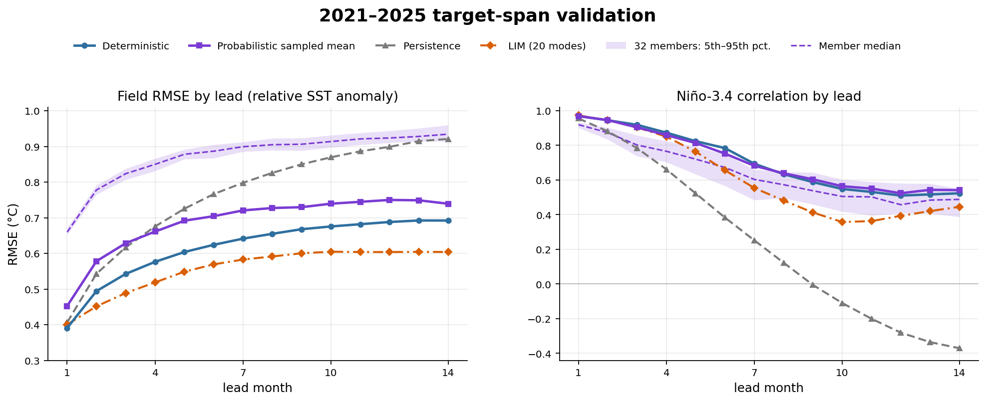
Table 3 collects the central point-forecast comparison; Table 4 attaches moving-block bootstrap intervals to the paired differences; Table 5 summarizes the ensemble metrics before and after calibration. Figure 4 resolves the deterministic and probabilistic center metrics by lead.

Metric (47 windows, 14 leads)	Persistence	Zero anomaly	Deterministic	Prob. sampled mean
Field RMSE (${}^{\circ}\mathrm{C}$)	0.779	0.654	0.622	0.692
Field ACC	0.302	—	0.415	0.406
Niño-3.4 RMSE (${}^{\circ}\mathrm{C}$)	0.914	0.785	0.541	0.651
Niño-3.4 correlation, leads 3–14	0.119	—	0.662	0.665

Difference (deterministic $-$ comparand)	Metric	Delta	90% CI	Status
vs. persistence	field RMSE (${}^{\circ}\mathrm{C}$)	$-0.157$	$[-0.244,\,-0.080]$	resolved
vs. zero anomaly	field RMSE (${}^{\circ}\mathrm{C}$)	$-0.032$	$[-0.055,\,-0.011]$	resolved
vs. sampled mean	field RMSE (${}^{\circ}\mathrm{C}$)	$-0.070$	$[-0.086,\,-0.048]$	resolved
vs. persistence	field ACC (per-window)	$+0.116$	$[-0.007,\,+0.261]$	unresolved
vs. persistence	Niño-3.4 corr., leads 3–14	$+0.544$	$[+0.080,\,+0.982]$	resolved
vs. sampled mean	Niño-3.4 corr., leads 3–14	$-0.003$	$[-0.017,\,+0.020]$	unresolved

Niño-3.4 ensemble metric (leads 3–14, LOYO)	Raw	Calibrated
Fair CRPS (${}^{\circ}\mathrm{C}$)	0.424	0.399
Spread–skill ratio	0.422	0.958
Central 50% coverage (nominal 50%)	29.3%	53.0%
Central 80% coverage (nominal 80%)	47.3%	66.7%
Central 90% coverage (nominal 90%)	54.4%	71.8%

The deterministic model satisfies every predeclared criterion. Its pooled relative-anomaly field RMSE is $0.622\,{}^{\circ}\mathrm{C}$, against $0.779\,{}^{\circ}\mathrm{C}$ for anomaly persistence and $0.654\,{}^{\circ}\mathrm{C}$ for a zero-anomaly forecast. Mean field ACC is $0.415$, mean leads-3–14 Niño-3.4 correlation is $0.662$, and Niño-3.4 RMSE is $0.541\,{}^{\circ}\mathrm{C}$. All outputs are finite and non-collapsed, the normalizer is unchanged from its training-only fit, and the deterministic tensors embedded in the probabilistic model remain bit-identical. Leadwise RMSE grows smoothly with lead rather than collapsing to a fixed climatological state (Figure 4); the deterministic curve is below persistence at all 14 leads and below the probabilistic sampled mean at every lead, while the unscaled LIM curve is below the deterministic curve at every lead except lead 1.

Under the paired moving-block bootstrap (Table 4), the RMSE margins over persistence ($-0.157\,{}^{\circ}\mathrm{C}$) and over the zero-anomaly forecast ($-0.032\,{}^{\circ}\mathrm{C}$) are resolved on this record, as is the Niño-3.4 correlation margin over persistence; the per-window field-ACC margin over persistence is not resolved. The modest resolved margin over the zero-anomaly forecast is worth emphasis: much of the large persistence gap reflects the degradation of persistence at long leads rather than large absolute skill.

The stronger statistical references of Section 5.2 sharpen this picture considerably (Table 6). The damped statistical forecasts attain lower pooled field RMSE than the deterministic model—the margins are resolved for the EOF ridge ($0.589\,{}^{\circ}\mathrm{C}$) and the LIM ($0.559\,{}^{\circ}\mathrm{C}$), and the LIM's per-window ACC advantage ($0.506$ versus $0.407$) is resolved as well. Their forecast amplitudes are strongly damped (spatial-variability ratios $0.37$–$0.51$ versus $0.72$ for the deterministic model and $1$ for the observations)—the climatology-like behavior that squared-error metrics reward—but the rescaling analysis shows that amplitude alone does not explain the gap. Because correlations are invariant to positive per-lead rescaling, amplitude is a free dial for the LIM: rescaled globally to the deterministic model's own amplitude ratio of $0.72$, the LIM still attains lower pooled RMSE, resolved on this record ($0.574$ versus $0.622\,{}^{\circ}\mathrm{C}$, difference $+0.048$, CI $[+0.024,\,+0.074]$), and only when pushed to near-observed amplitude by the training-fitted restoration (validation ratio $0.93$) does its advantage dissolve into an unresolved difference ($0.631$ versus $0.622\,{}^{\circ}\mathrm{C}$, CI $[-0.054,\,+0.038]$). Amplitude retention is therefore not by itself a distinguishing property of the learned model. What remains distinguishing on this record is the leads-3–14 Niño-3.4 correlation, where the deterministic model is highest among the single-trajectory forecasts ($0.662$ versus $0.550$ for the LIM at any rescaling; the probabilistic sampled mean matches it at $0.665$); that margin is concentrated at leads 7–14 (Figure 4) but is not resolved at the house block length. Stated plainly: on bulk field metrics the LIM family is at least as good as the deterministic model across the evaluated amplitude scalings, and the learned model's demonstrated edge is confined to long-lead index coherence, achieved without any post-hoc variance tuning, with a margin this record cannot resolve.

Stratifying by initialization season yields mean leads-3–14 Niño-3.4 correlations between $0.625$ (JJA starts) and $0.665$ (DJF starts); with only ${\sim}12$ overlapping windows per season these values are descriptive, but no dramatic seasonal collapse is visible in this record. For orientation only: simulation-pretrained deep-learning ENSO systems have reported all-season Niño-3.4 correlation skill above $0.5$ to roughly 17-month leads on multi-decade hindcast periods [1]. Such values are not comparable to Table 6—the verification periods, anomaly and climatology conventions, and train–test protocols all differ, and the present record consists of 47 overlapping windows dominated by two ENSO episodes—so no cross-study ranking is implied, and no comparison against operational ENSO forecast systems is claimed (Section 7).

Reference	Field RMSE	$\Delta$ RMSE (90% CI)	ACC (pw)	Niño-3.4 corr. 3–14	Ampl. ratio
Persistence	0.779	$-0.157$ $[-0.244,-0.080]$	0.291	0.119	1.02
Zero anomaly	0.654	$-0.032$ $[-0.055,-0.011]$	—	—	0
Damped persistence	0.604	$+0.018$ $[-0.001,+0.036]$	0.291	0.119	0.37
EOF ridge (20 modes)	0.589	$+0.033$ $[+0.007,+0.057]$	0.430	0.580	0.44
LIM (20 modes)	0.559	$+0.063$ $[+0.043,+0.081]$	0.506	0.550	0.51
LIM, amplitude-restored	0.631	$-0.009$ $[-0.054,+0.038]$	0.506	0.550	0.93
Deterministic model	0.622	—	0.407	0.662	0.72
Prob. sampled mean	0.692	$-0.070$ $[-0.086,-0.048]$	0.388	0.665	0.75

Two predeclared single-factor ablations of the frozen recipe address the attribution question directly. Removing the CMIP6 forecast-pretraining overlay (retaining the underlying Earthformer base weights, the freeze boundary, the objective, and the selection rule) produced no checkpoint satisfying the predeclared selection guards, at either the budget-matched 1,000 updates or a budget-extended run (up to 4,000 updates; early-stopped with degrading skill): the best persistence improvement reached was $-0.015\,{}^{\circ}\mathrm{C}$ (never better than persistence) and the best leads-3–14 Niño-3.4 correlation was $0.29$, against $0.662$ for the full model. The CMIP6 pretraining is therefore necessary for skill beyond persistence under this recipe, and training budget is not the explanation. The second ablation—removing the persistence-residual anchor in favor of direct coefficient forecasting—is structurally unavailable as a single-factor change: the training objective requires residual targets by construction, so the residual formulation's contribution cannot be isolated without also changing the objective; we report this coupling rather than substituting a different loss. Representation ablations (lowpass-only, field-space) and a full-capacity from-scratch model remain future work (Section 7).

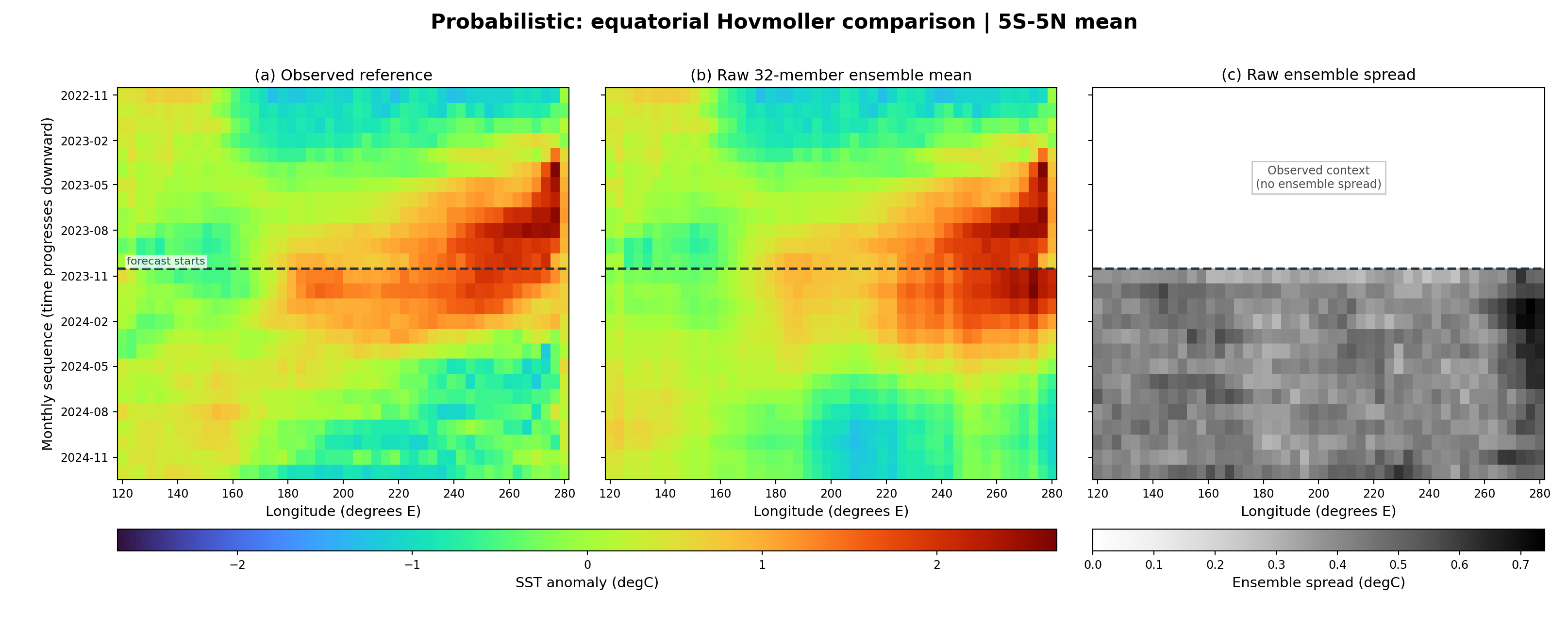
The raw ensemble's behavior divides into what it delivers, what it costs, and what remains uncalibrated. It delivers 32 distinct finite members with nonzero spread whose coefficient bands reconstruct the saved member fields to numerical tolerance, an all-lead Niño-3.4 fair CRPS of $0.385\,{}^{\circ}\mathrm{C}$, and a sampled mean that stays in the learned-forecast family of Table 6: amplitude ratio $0.75$ and leads-3–14 Niño-3.4 correlation $0.665$ (the difference from the deterministic center's $0.662$ is unresolved). It costs a center displacement: the sampled 32-member mean is worse than the deterministic forecast on all three center metrics—field RMSE $0.692$ versus $0.622\,{}^{\circ}\mathrm{C}$ (resolved, $-0.070\,{}^{\circ}\mathrm{C}$; Table 4), field ACC $0.406$ versus $0.415$, and Niño-3.4 RMSE $0.651$ versus $0.541\,{}^{\circ}\mathrm{C}$—so the predeclared center-adoption criterion is not met. What remains uncalibrated is quantified below and in Section 6.4.

Ten additional 32-member ensembles, generated from the frozen checkpoint under predeclared sampling seeds after the canonical evaluation, show that this center displacement is systematic rather than Monte Carlo noise. Every replication's sampled mean is worse than the deterministic center on all three metrics (replication field RMSE spans a narrow $0.690$–$0.693\,{}^{\circ}\mathrm{C}$), and pooling all 352 saved members plateaus at field RMSE $0.685\,{}^{\circ}\mathrm{C}$ and Niño-3.4 RMSE $0.640\,{}^{\circ}\mathrm{C}$—closer to, but still clearly short of, the deterministic values ($0.622$ and $0.541\,{}^{\circ}\mathrm{C}$; in the per-window ACC convention, $0.397$ pooled versus $0.407$ deterministic). The learned residual distribution is therefore not centered on the deterministic trajectory, and larger ensembles cannot close the gap. These replications are sensitivity evidence only; the canonical seed-42 ensemble remains the frozen product.

The temporal diagnostics localize where sampled trajectories depart from observed behavior. Lowpass lag retention is $0.838$, above the $0.608$ structural floor, so member trajectories do retain most of the observed month-to-month continuity in the lowpass band. However, the trajectory-dispersion ratio is $1.315$ (member Niño-3.4 trajectories change 31% more from month to month than observed ones; the ten seed replications span $1.290$–$1.313$, so the canonical realization is the most dispersive), and the member high-frequency power fraction is $0.580$ versus $0.423$ in the observations. Flow dependence is $-0.161$ in the canonical realization, but the seed replications qualify this value: it spans $-0.16$ to $+0.22$ across the eleven realizations and is centered near zero, so the robust statement is not that spread is anti-correlated with error but that this diagnostic is seed-noise-dominated at 47 windows and spread carries no detectable flow-dependent signal on this record. Taken together, these diagnostics indicate that the head injects too much temporally unstructured variability—consistent with sampling noise independently across leads ($\rho=0$)—rather than state-dependent uncertainty.

On the calibration lead scope (leads 3–14), spread-only leave-one-year-out calibration improves Niño-3.4 fair CRPS from $0.424$ to $0.399\,{}^{\circ}\mathrm{C}$ and raises spread–skill from $0.422$ to $0.958$. The near-unit spread–skill is largely guaranteed by the error-variance-matching fit of Section 4.3; the informative outcome is the coverage. Central 50/80/90% coverage becomes $53.0/66.7/71.8\%$: the 50% interval is within the 10-point tolerance, but the 80% and 90% intervals under-cover by 13 and 18 points. Matching the second moment is therefore not sufficient, which implicates the distribution's shape—tails, conditional heteroscedasticity, or the temporal dependence that ECC-Q deliberately carries over from the raw ensemble—and the displaced center. ECC-Q rank preservation and the ensemble-mean identity hold exactly.

Two predeclared sensitivity variants separate those causes. First, adding a leave-one-year-out per-lead mean correction to the spread-only calibration—the same parameter count per lead as $\sigma_{\ell}$—does not repair the product: fair CRPS moves only from $0.399$ to $0.395\,{}^{\circ}\mathrm{C}$ while spread–skill collapses to $0.767$ and 50/80% coverage falls to $25.5/55.0\%$. The fitted per-lead biases are large ($-0.1$ to $-0.6\,{}^{\circ}\mathrm{C}$) but differ across the four context-start-year folds, so a stationary mean correction does not transfer across held-out years; this empirically supports leaving the sampled center untouched in the frozen product. Second, recentering the archived member deviations on the frozen deterministic trajectory—no fitting at all—improves fair CRPS from $0.399$ to $0.325\,{}^{\circ}\mathrm{C}$, restores spread–skill $0.957$, and raises 80/90% coverage to $70.7/79.4\%$ (50%: $42.4\%$). Most of the calibrated shortfall is therefore attributable to the displaced sampled center rather than to the noise shape alone, which quantifies the value of the mean-preserving sampling requirement stated in Section 7. Both variants are sensitivity evidence only; the archived spread-only calibration remains the frozen product.

The lowpass lifting reproduces its algebraic identities numerically: lifted member indices match their calibrated trajectories to below $5.1\times10^{-7}\,{}^{\circ}\mathrm{C}$, the ensemble-mean field shifts by less than $4.8\times10^{-7}\,{}^{\circ}\mathrm{C}$, and highpass coefficients are unchanged (band-energy changes below 0.23%). A supplementary member-field spread-ratio check moves from $1.132$ to $1.211$, exceeding its declared $0.05$ tolerance; this reflects the calibrated index spread materializing in the member fields, and does not alter the exact index, mean, or highpass assertions.

Under Eq. (9), the deterministic background-restored field RMSE is $0.647\,{}^{\circ}\mathrm{C}$, background-restored Niño-3.4 correlation is $0.762$, and three-month ONI-style RMSE is $0.609\,{}^{\circ}\mathrm{C}$. The lifted probabilistic ensemble obtains background-restored leave-one-year-out fair CRPS $0.391\,{}^{\circ}\mathrm{C}$, spread–skill $0.896$, pooled ONI-style correlation $0.772$, pooled ONI-style RMSE $0.685\,{}^{\circ}\mathrm{C}$, and a mean El Niño/La Niña event Brier score of $0.203$. Judged against a per-calendar-month climatological probability forecast fitted on 1981–2020 in the same index frame (mean event Brier $0.219$; a pooled-base-rate variant scores $0.225$), that mean corresponds to a Brier skill score of only $+0.07$, and the mean conceals a strong asymmetry: the El Niño score is $0.089$ (skill score $+0.54$) while the La Niña score is $0.317$ (skill score $-0.30$, worse than climatology). The La Niña failure is consistent with the persisted warm context-end tropical-mean background during the 2021–2022 La Niña episode, and it cautions against reading the mean event Brier as uniform event skill. All background-restored values are conditional on the context-end tropical-mean persistence assumption and are not comparable to indices computed against a centered operational climatology.

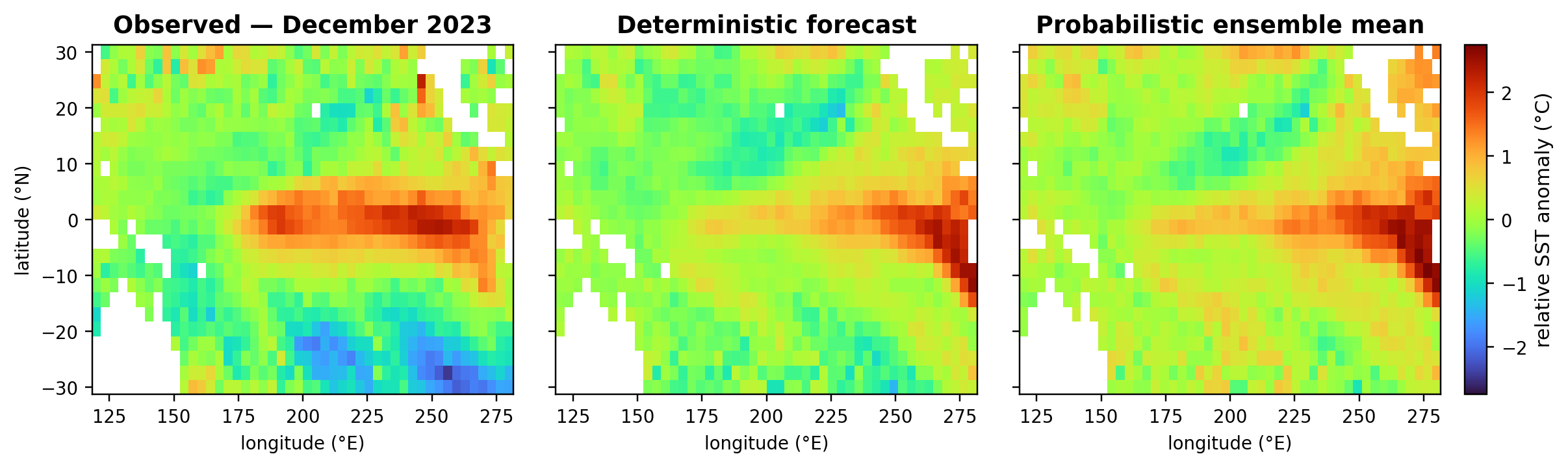
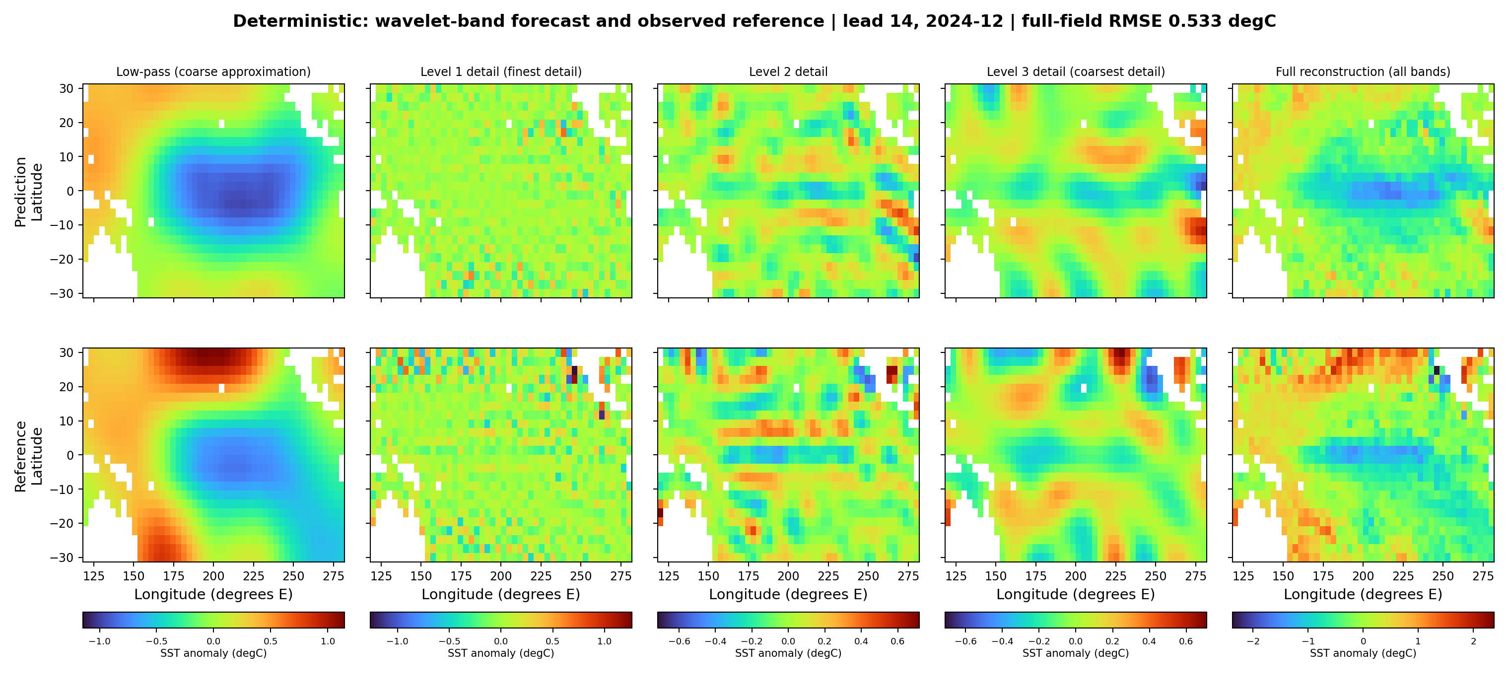
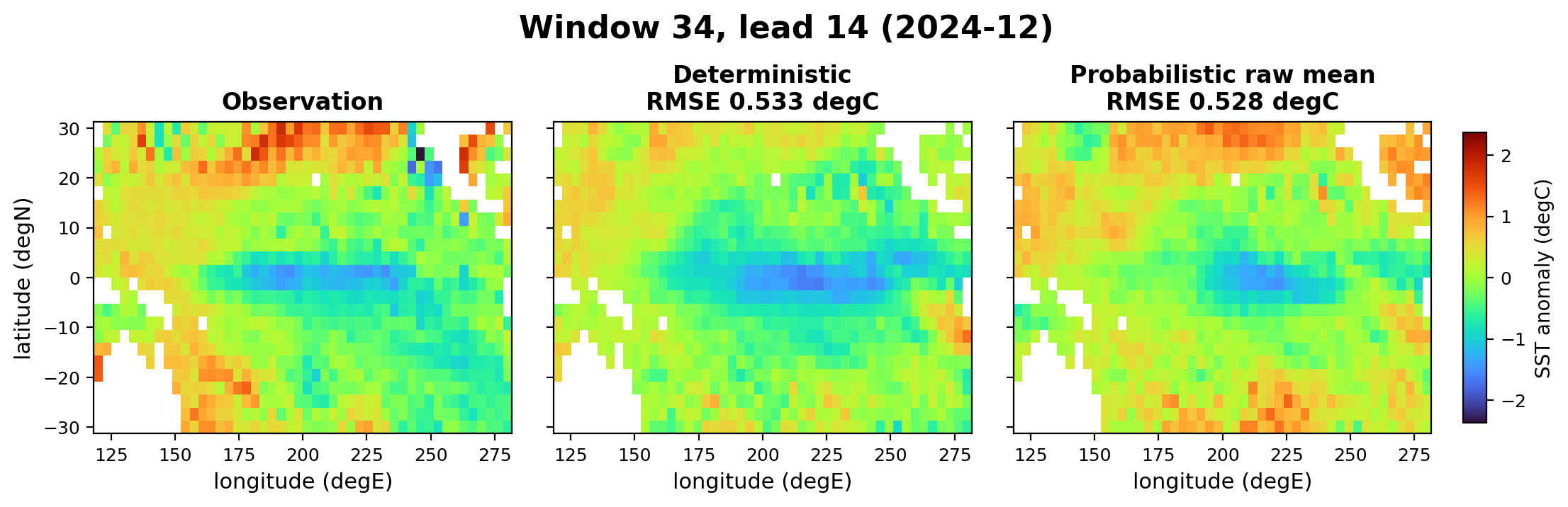
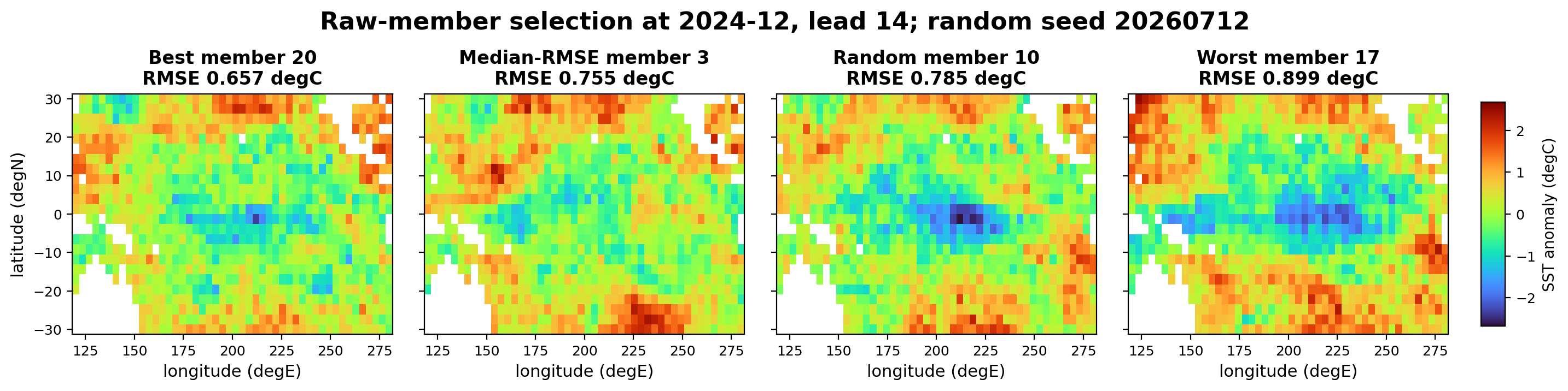
The complete validation gallery contains deterministic and probabilistic renderings for every window. The title-page graphic is selected by a separate, event-timed rule: the target month with the maximum verifying Niño-3.4 index of the 2023–24 El Niño (December 2023, $+1.42\,{}^{\circ}\mathrm{C}$ in the relative frame), shown at lead 4 (window 32, context ending August 2023). That rule uses only the observed event timing, not forecast skill; the case's field RMSEs ($0.635\,{}^{\circ}\mathrm{C}$ deterministic, $0.758\,{}^{\circ}\mathrm{C}$ sampled mean) are worse than the pooled values of Table 3, so the cover is not a favorable selection. For the body figures, a predeclared display rule restricts attention to five evenly spaced windows (0, 12, 23, 34, 46) and, within those, selects the window minimizing full-field reconstruction RMSE (for the deterministic decomposition, also the mean RMSE across the lowpass and three detail levels). Both rules select window 34, whose lead-14 target is December 2024—a favorable case for both models by construction. These display choices are for illustration only and do not affect checkpoint choice or any aggregate score. Within the saved raw ensemble for this target, the best, median-error, and worst members are identified by valid-cell full-field RMSE against the verifying observation—a hindsight selection that could not be made in real time and is used only to visualize the ensemble's range—and one member is drawn at random under a fixed seed as a verification-independent view.

What the deterministic result shows. The deterministic model improves substantially on anomaly persistence while retaining positive spatial and index association, with leadwise error growing smoothly through lead 14—but the statistical references bound the claim tightly: a 20-mode LIM fitted on the same training partition beats it on pooled field RMSE and per-window ACC, retains a resolved RMSE advantage even when rescaled to the deterministic model's own amplitude, and only loses that advantage (to an unresolved difference, not a deficit) when rescaled to near-observed amplitude. The model's demonstrated value is therefore not bulk error minimization and not amplitude per se; it is long-lead index coherence—the highest leads-3–14 Niño-3.4 correlation among single-trajectory forecasts, achieved without post-hoc variance tuning—and that margin is itself unresolved on this record (Section 6.1). This is a development-validation result: the 2021–2025 windows served for both checkpoint selection and scoring, so generalization to an untouched period has not been measured. The ablations attribute the skill only partially: CMIP6 pretraining is necessary under this recipe (Section 6.2), but the contributions of the wavelet representation and the persistence-residual formulation remain untested—the latter because it is structurally inseparable from the training objective—and comparisons with operational ENSO prediction systems—which assimilate subsurface and wind information unavailable to this SST-only model—are out of scope for the present record. At 6–14 month leads, subsurface heat content and wind forcing carry substantial predictive information, so the SST-only setting should be read as a deliberately constrained forecast problem.

What the probabilistic characterization shows. The probabilistic model generates a nondegenerate, reproducible ensemble and retains most lowpass temporal continuity; its sampled mean carries a systematic displacement on all three center metrics, its spread is uninformative about error (no detectable flow-dependent signal on this record), and its trajectories carry excess high-frequency variability. Spread-only calibration repairs the overall width (spread–skill $0.958$) and improves fair CRPS, yet 80/90% intervals still under-cover, indicating a distribution-shape mismatch that a single per-lead width cannot fix and that rank-preserving ECC-Q, by design, carries over from the raw ensemble. The lifting step faithfully implements the requested index calibration but cannot alter the underlying sequence distribution. These findings indicate that independent-across-lead noise injection around a frozen center supplies marginal width but not the temporal dependence or truth-centered mean of monthly ENSO trajectories, and they specify the requirements for the next design axis: temporally correlated, state-conditional, mean-preserving sampling. The calibration sensitivity variants of Section 6.4 put numbers on the mean-preserving requirement: recentering the archived deviations on the deterministic trajectory improves cross-validated development-period fair CRPS from $0.399$ to $0.325\,{}^{\circ}\mathrm{C}$ and lifts 80/90% coverage to $70.7/79.4\%$, whereas a fitted per-lead mean correction fails to transfer across context-start years. The seed-replication analysis of Section 6.3 settles the earlier ambiguity about the center metrics: the displacement is systematic, not Monte Carlo noise. It also shows that the flow-dependence statistic itself is seed-noise-dominated on 47 windows, so single-realization values of that diagnostic—in this or any comparable study—should be interpreted with caution. Under the predeclared adoption rule, the probabilistic product was not adopted.

Evaluation-design limitations. The 47 windows overlap and verify only 60 unique months dominated by two ENSO episodes. Pooled comparisons carry moving-block bootstrap intervals (Table 4), and the block-length sensitivity of Section 5.1 shows the resolved/unresolved labels are stable for blocks of 3–14 windows, but only about four independent year-blocks support them, so the intervals remain approximate; the leave-one-year-out calibration folds likewise share verifying months across fold boundaries (Section 4.3); and the initialization-season stratification is descriptive and coarse, so fine-grained spring-predictability-barrier structure remains unresolved. The record is short, the grid coarse, and the acceptance criteria—although fixed in version-controlled planning documents before the runs—are project-defined rather than externally registered. The warm-up climatology makes early training anomalies non-causal with respect to real-time availability (Section 3.1), reference discontinuities at five-year block boundaries can inject artificial shifts into windows that straddle them, and zero-filling land cells before the DTCWT contaminates coefficients whose spatial support overlaps coastlines, an effect mitigated but not eliminated by valid-cell masking of the field-space losses and scores. Background-restored results additionally assume persistence of the context-end tropical-mean departure; rapid background changes violate that assumption, and the event-score decomposition of Section 6.4—El Niño exceedances far better than climatology, La Niña exceedances worse than climatology—is the concrete signature of that violation on this record.

On a 2021–2025 development-validation period, a deterministic complex-wavelet Earthformer with CMIP6 pretraining, a persistence-residual formulation, and restricted observational fine-tuning outperformed relative-anomaly persistence at every lead (field RMSE $0.622$ versus $0.779\,{}^{\circ}\mathrm{C}$, and $0.654\,{}^{\circ}\mathrm{C}$ for a zero-anomaly forecast; both margins resolved under a paired moving-block bootstrap and stable across bootstrap block lengths) while retaining positive spatial and Niño-3.4 association; its generalization to an untouched period has not yet been measured. Statistical references bound the claim: a 20-mode linear inverse model attains lower pooled field RMSE ($0.559\,{}^{\circ}\mathrm{C}$), retains a resolved advantage when rescaled to the learned model's amplitude ($0.574\,{}^{\circ}\mathrm{C}$), and is only reduced to statistical parity at near-observed amplitude, so the learned model's demonstrated contribution narrows to the highest long-lead Niño-3.4 correlation among single-trajectory forecasts—a margin this record cannot resolve— achieved without post-hoc variance tuning; an ablation shows this skill depends causally on the CMIP6 pretraining, without which no checkpoint beat persistence. The residual-diffusion ensemble built around that frozen center produced finite, nondegenerate, fully archived members in the same learned-forecast family—near-observed amplitude and matching index correlation—at the cost of a systematic center displacement confirmed across ten sampling-seed replications and 352 pooled members, with no detectable flow-dependent error–spread association on this record, excess high-frequency trajectory variability, and calibrated 80/90% intervals that remain under-dispersive. The ensemble is characterized rather than adopted: its center displacement and dependence structure define the requirements—temporally correlated, state-dependent, and mean-preserving sampling—that any successor generative head must meet, and the sensitivity analysis quantifies the largest single prize: recentering alone would improve cross-validated development-period fair CRPS from $0.399$ to $0.325\,{}^{\circ}\mathrm{C}$. The natural next steps are confirmatory evaluation on a sealed post-2025 period, representation ablations and comparison with operational ENSO prediction systems, and a generative head meeting the requirements above.

ERA5 monthly-mean SST was obtained from the Copernicus Climate Change Service (C3S) Climate Data Store [2]. CMIP6 historical tos fields were obtained through the Pangeo/ESGF Google Cloud CMIP6 catalog; the model list is given in Section 4.1. The Earthformer base weights are the publicly released ICAR-ENSO checkpoint accompanying [5]. The training and evaluation pipeline, the configuration files and validation protocol that fix the acceptance criteria, the reference scorecards, and the scripts that regenerate every reported result and figure are openly available in a public code repository (https://github.com/not-JASH/Complex-Wavelet-Earthformer-ENSO). The large binary artifacts—the canonical raw 32-member ensemble, the ten seed-replication stores, the calibrated and lifted member fields, and the trained checkpoints—are archived, with SHA-256 manifests, in a Zenodo deposit (https://doi.org/10.5281/zenodo.21423063).

This work used ERA5 data generated using Copernicus Climate Change Service information (2026); neither the European Commission nor ECMWF is responsible for any use of this information. We acknowledge the World Climate Research Programme's Working Group on Coupled Modelling, the climate modeling groups listed in Section 4.1 for producing and sharing their CMIP6 output, and the Earth System Grid Federation and Pangeo for data access. We thank the Earthformer authors for releasing the ICAR-ENSO checkpoint used as the backbone initialization.

Notes

1. Training models: CESM2, CESM2-FV2, CESM2-WACCM, CESM2-WACCM-FV2, E3SM-1-0, E3SM-1-1, E3SM-1-1-ECA, GFDL-CM4, GISS-E2-1-G, GISS-E2-1-G-CC, GISS-E2-1-H. Held out for checkpoint selection: GFDL-ESM4, MCM-UA-1-0, MRI-ESM2-0. All are historical r1i1p1f1 realizations, one per source. Back
2. Internal objective identifier residual_skill_v0; the correlation and index terms exist because RMSE alone rewards damped, climatology-like forecasts. Back

References

- Y.-G. Ham, J.-J. Kim, and J.-J. Luo, “Deep learning for multi-year ENSO forecasts,” Nature, 573:568–572, 2019.
- H. Hersbach et al., “The ERA5 global reanalysis,” Quarterly Journal of the Royal Meteorological Society, 146:1999–2049, 2020.
- N. Kingsbury, “Complex wavelets for shift invariant analysis and filtering of signals,” Applied and Computational Harmonic Analysis, 10(3):234–253, 2001.
- I. W. Selesnick, R. G. Baraniuk, and N. G. Kingsbury, “The dual-tree complex wavelet transform,” IEEE Signal Processing Magazine, 22(6):123–151, 2005.
- Z. Gao et al., “Earthformer: Exploring space-time transformers for Earth system forecasting,” in Advances in Neural Information Processing Systems, vol. 35, 2022.
- V. Eyring et al., “Overview of the Coupled Model Intercomparison Project Phase 6 (CMIP6) experimental design and organization,” Geoscientific Model Development, 9:1937–1958, 2016.
- S. Rasp and N. Thuerey, “Data-driven medium-range weather prediction with a ResNet pretrained on climate simulations: A new model for WeatherBench,” Journal of Advances in Modeling Earth Systems, 13:e2020MS002405, 2021.
- M. Mardani et al., “Residual corrective diffusion modeling for km-scale atmospheric downscaling,” arXiv:2309.15214, 2023.
- I. Price et al., “Probabilistic weather forecasting with machine learning,” Nature, 637:84–90, 2025.
- J. Ho, A. Jain, and P. Abbeel, “Denoising diffusion probabilistic models,” in Advances in Neural Information Processing Systems, vol. 33, 2020.
- J. Ho, T. Salimans, A. Gritsenko, W. Chan, M. Norouzi, and D. J. Fleet, “Video diffusion models,” in Advances in Neural Information Processing Systems, vol. 35, 2022.
- T. Gneiting, A. E. Raftery, A. H. Westveld, and T. Goldman, “Calibrated probabilistic forecasting using ensemble model output statistics and minimum CRPS estimation,” Monthly Weather Review, 133:1098–1118, 2005.
- R. Schefzik, T. L. Thorarinsdottir, and T. Gneiting, “Uncertainty quantification in complex simulation models using ensemble copula coupling,” Statistical Science, 28(4):616–640, 2013.
- C. A. T. Ferro, “Fair scores for ensemble forecasts,” Quarterly Journal of the Royal Meteorological Society, 140:1917–1923, 2014.
- T. Gneiting and A. E. Raftery, “Strictly proper scoring rules, prediction, and estimation,” Journal of the American Statistical Association, 102:359–378, 2007.
- M. L. L'Heureux et al., “A relative sea surface temperature index for classifying ENSO events in a changing climate,” Journal of Climate, 37(4):1197–1211, 2024.
- T. Izumo et al., “Relevance of relative sea surface temperature for tropical rainfall interannual variability,” Geophysical Research Letters, 47, e2019GL086182, 2020.
- C. Penland and P. D. Sardeshmukh, “The optimal growth of tropical sea surface temperature anomalies,” Journal of Climate, 8(8):1999–2024, 1995.
- NOAA Climate Prediction Center, “Oceanic Niño Index changes description: centered 30-year base periods updated every five years,” 2017, https://www.cpc.ncep.noaa.gov/products/analysis_monitoring/ensostuff/ONI_change.shtml.