Building and Validating a Complex-Wavelet Earthformer Forecasting System
Scientific Report 1: Data, Representation, Integration, and Validity Gates
Abstract
This is a methods-validation study; every outcome in it is engineering evidence (E0-ENG) and none is a forecast-skill claim. We construct and validate a leakage-safe pipeline from monthly tropical-Pacific sea-surface temperature (SST), through a complete three-level dual-tree complex wavelet (DTCWT) coefficient pyramid, into the official Earthformer architecture with the released ICAR-ENSO checkpoint, and back through exact inverse transforms to reconstructed forecast maps and Hovmöller products. The validated contracts are: bitwise-lossless coefficient packing; numerically verified inverse reconstruction; recorded, reversible dense-grid lifting with channel-aligned validity masks; shape-safe checkpoint surgery with deterministic load reports (173/177 official tensors reused in coefficient-native mode); declared gradient boundaries (all fresh tensors receive gradients, maximum frozen gradient exactly zero); exact checkpoint save/reload roundtrips; split-contained preprocessing in which climatology and normalization statistics are fit on training timestamps only; and fail-closed data access under which sealed test months are never materialized. Bounded one-batch and small real-data optimizations demonstrate trainability only. Predictive adequacy is deliberately deferred to Report 2.
1. Study Identity and Handoff
Study ID R1. Incoming state: a project concept and the released ICAR-Earthformer checkpoint. Changed factor: construction of the full coefficient-domain forecasting system. Evidence tier: E0-ENG (engineering and bounded optimization only). Outgoing artifact: a validated data/model/evaluation boundary — chronological splits, lossless representation, integrated official backbone, checkpoint and normalization contracts — that Report 2 uses for controlled scientific ablations. Timeline: work recorded 2026-06-28 through 2026-06-30; no observed validation consultation and no test access occur in this study.
2. Introduction
Monthly tropical-Pacific SST anomaly fields carry the spatial structure that distinguishes ENSO flavors and drives teleconnections; forecasting the field, rather than an index, preserves that structure for downstream use. Multiscale, oriented representations are natural for such fields: anomaly patterns have basin-scale envelopes, frontal edges, and oriented equatorial structure at different scales. The dual-tree complex wavelet transform offers near-shift-invariance and six oriented complex subbands per level at $4:1$ redundancy in 2-D [1, 2], and modern spatiotemporal transformers such as Earthformer [3] provide strong sequence-to-sequence backbones for gridded geophysical data.
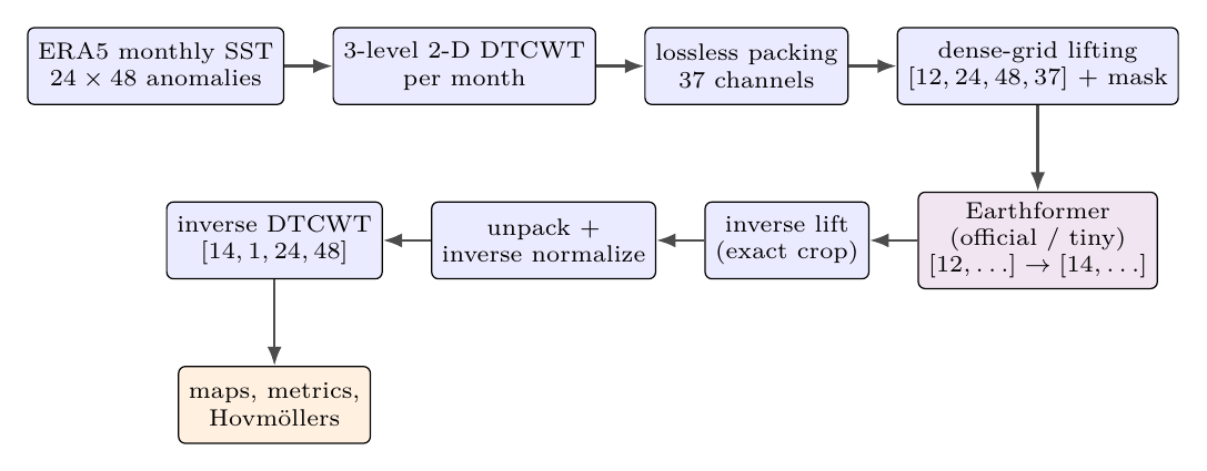
The methodological question this report answers is narrow and prior to any skill question: can a complete 2-D DTCWT representation of monthly SST be passed through an Earthformer-style forecast model without losing invertibility, provenance, or leakage control? “Complete” is load-bearing — the system retains every coefficient of every level, so any forecast in coefficient space maps exactly to a physical field. The report documents the contracts that make that true and the gate evidence that each contract holds.
2.1 Contributions
- A staged ERA5 pipeline (download, standardize, regrid, anomalies, split, coefficients, normalize) with atomic retrieval, manifests, and JSON reports.
- A complete 37-channel DTCWT schema: one lowpass plus $3\times(6\times2)$ oriented real/imaginary highpass channels per monthly map.
- Bitwise-lossless native pyramid packing plus a recorded, exactly invertible dense-grid lifting with channel-aligned validity masks.
- Official-model integration through auditable checkpoint surgery with deterministic load reports; no silent fallback to the tiny smoke backbone and no silent CUDA-to-CPU downgrade.
- A persistence-initialized synthetic vertical slice exercising the whole chain end to end.
- Versioned checkpoint and normalization contracts with exact-reload verification and embedded provenance.
- Deterministic evaluation products (per-window metrics, lead plots, map panels, Hovmöller diagrams) and fail-closed data gates.
Deep ENSO forecasting entered the literature with CNN index regression pretrained on CMIP simulations [4]; Earthformer moved the target to gridded fields, publishing an ICAR-ENSO configuration and pretrained checkpoint with a 12-month context and 14-month future decoder on a $24\times48$ grid [3]. We adopt that exact geometry so the released checkpoint's positional and attention structure remains valid.
Wavelet representations have a long record in geophysical analysis, and complex wavelets specifically address the shift-sensitivity of critically sampled DWTs [1]. In deep learning they appear both as fixed front-ends and as analysis tools [6]. Coefficient-domain forecasting — predicting the transform of a future field rather than the field — is attractive here for three reasons: (i) the transform isolates scale and orientation, enabling scale-selective losses and diagnostics later in the series; (ii) the lowpass band concentrates the basin-scale signal that regional indices read; (iii) invertibility keeps physical-space evaluation exact. The design choice validated in this report is a spatial DTCWT applied independently per month, with time handled entirely by the sequence backbone: months are never mixed by the transform, so temporal leakage through the representation is structurally impossible. We make no claim in this report that the wavelet representation is superior to map-space modeling; no comparison is run here.
4. Data and Preprocessing Contract
Version 0 uses ERA5 monthly averaged single-level SST [5] retrieved from the Copernicus Climate Data Store as NetCDF. Preprocessing stages are:
- standardize: rename coordinates, convert longitudes to $0$–$360^\circ$ and sort, crop the domain, aggregate to month starts, convert Kelvin to Celsius;
- regrid: linear interpolation onto the endpoint-inclusive $24\times48$ grid over $30^{\circ}$S–$30^{\circ}$N, $120^{\circ}$E–$280^{\circ}$E;
- anomalies: fit a 12-calendar-month climatology on the configured reference interval and store climatology and anomalies separately;
- split: construct chronological, split-contained 12-month-context to 14-month-target windows;
- coefficients: zero-fill missing cells only at the DTCWT boundary, save the map validity mask and the native real/imaginary pyramid, and verify inverse-DTCWT reconstruction;
- normalize: fit mask-aware streaming per-channel statistics on training months only and apply the frozen statistics to all partitions.
Because CDS payloads cannot cross the $180^\circ$ meridian in one request, the production profile (1981–2020) issues 16 bounded requests — eight five-year time chunks $\times$ two longitude regions — writes an aggregate manifest before retrieval, then merges, deduplicates the $180^\circ$ seam, and validates a unique, strictly increasing longitude coordinate covering $120$–$280^{\circ}$E. A deliberately tiny two-year smoke request (24 monthly maps, west Pacific only, validated 2026-06-29) exercises the mechanics; it is distinguished everywhere from the scientific record, and because 24 months cannot contain one 26-month window, its window construction correctly reports zero windows and normalization is skipped.
4.1 Chronology and Leakage Prevention
The v0 chronology is: training 1981-01–2010-12, validation 2011-01–2015-12, test 2016-01–2020-12 (Table 1). Windows are wholly contained in their split; a window whose 26 months would cross a boundary is excluded. Two leakage controls are structural rather than procedural: the anomaly climatology interval must be contained in the training interval, and the coefficient normalizer selects unique training timestamps before fitting, applying one frozen versioned schema to all partitions. Test-month chunks are not materialized during development; the shared supervised loader fails closed at 2015-12, and every training and evaluation artifact records test_data_read: false.
| Partition | Span | Months | Windows | Access policy |
|---|---|---|---|---|
| Training | 1981-01–2010-12 | 360 | 335 | climatology and normalizer fit here only |
| Validation | 2011-01–2015-12 | 60 | 35 | consulted by later reports (E3-VAL) |
| Test | 2016-01–2020-12 | 60 | 35 | sealed; fail-closed, never materialized here |
4.2 Preprocessing Verification
The pipeline's validity gates (not predictive results) are: coordinate and unit checks (explicit Kelvin detection); calendar/month-start aggregation checks; duplicate-longitude detection at the seam; grid-coverage assertions; missing-value accounting with mask persistence; transform–reconstruction tolerance on real maps; timestamp-boundary audits immediately before array materialization; and manifest/report emission for every stage.
5. Complex-Wavelet Representation
Each monthly map $y_t \in \mathbb{R}^{24\times 48}$ is transformed independently by a three-level 2-D DTCWT:
with $L_t$ the real lowpass residual and six oriented complex subbands ($\pm15^\circ,\pm45^\circ,\pm75^\circ$) per level. The packer moves orientation and complex axes into channels,
and real/imaginary channels remain paired through normalization, loss computation, unpacking, and inverse reconstruction. For one SST channel and three levels the lifted grid has
5.1 Lossless Packing and Native Geometry
CoefficientPacker.pack preserves the complete inverse-reconstruction package: the real lowpass residual; every ordered native-resolution highpass level; channel, orientation, height, and width metadata per level; the original unpadded map geometry; and complex-encoding and channel-order identifiers. unpack restores the coefficient object exactly — packing neither interpolates nor merges scales, so pack/unpack is bitwise lossless. This serialization layer is deliberately separate from the model adapter that follows.
5.2 Dense-Grid Lifting
Pyramid levels have different spatial sizes; a conventional projection expects one regular grid. CoefficientGridLifter zero-pads every native component on its bottom/right edges to the largest level (or a configured larger grid, here $24\times48$ so the official positional embeddings apply exactly), concatenates channels, and records the strategy, grid size, component channel slices, native shapes, and exact padding tuples. Its inverse crops rather than resizes: an unchanged lifted tensor returns the bit-exact packed pyramid. Each lifted tensor carries a boolean validity mask with the same $[C,H,W]$ tail; with padded_mask_mode: apply the adapter multiplies both its input and output by this mask, so padded cells contribute exact zeros to any dense coefficient loss. This is a boundary/loss mask, not an internal attention mask: the official cuboid blocks expose no compatible token-mask argument at this boundary, so padded tokens may still influence valid tokens inside the model — a recorded limitation for later work, and one reason Report 2's ablations treat architecture-internal behavior as a variable.
5.3 Coefficient Normalization
CoefficientNormalizer fits streaming population mean/std statistics on native packed pyramids at scopes global, per_group, or the default per_channel (retaining level/orientation/real-imaginary distinctions). Optional boolean masks exclude cells from count, sum, and squared sum. The JSON/YAML metadata is schema-named and versioned and embeds the complete versioned packing metadata; loading or applying statistics against a different coefficient layout, channel order, encoding, level count, or spatial geometry raises an error rather than warning. Predictions are inverse-normalized before inverse DTCWT, so reconstructed-field losses and diagnostics remain in SST-anomaly units:
6. Earthformer Integration
The integration targets Amazon Science's official CuboidTransformerModel — a non-autoregressive channels-last encoder–decoder taking $[B,T_{\mathrm{in}},H,W,C_{\mathrm{in}}]$ to $[B,T_{\mathrm{out}},H,W,C_{\mathrm{out}}]$ — constructed with the published ICAR-ENSO options: 12 context months, 14-month future decoder, $24\times48$ grid, base width 64, two encoder/decoder scales, axial attention [3]. The official repository is kept in an external checkout (never vendored) because its published training environment pins an older stack; model-only import requires only einops. The local default is an explicit tiny fallback with the same tensor contract and persistence initialization — a smoke device, not cuboid attention — and official mode never falls back to it silently.
The initial integration used a project-owned one-channel bridge ($37\to1\to\mathrm{Earthformer}(1)\to1\to37$): the released one-channel boundary weights load into the unchanged official backbone while fresh project projections carry the coefficient channels, so released tensors are never misidentified as coefficient projections. The bridge validated the plumbing but is severely damping as a representation (Report 2) and is retained only for old-checkpoint compatibility. The primary mode, coefficient_native, constructs the official model directly at $[12,24,48,37]\to[14,24,48,37]$: the official first convolution embeds all 37 channels, the official head emits all 37, and a structural audit rejects any $37\to1$ module.
6.1 Checkpoint Surgery and Trainability
Checkpoint loading strips wrapper prefixes, filters tensor-shape mismatches before load_state_dict, and returns a deterministic CheckpointLoadReport of loaded, skipped (with reasons and shapes), missing, unexpected, and freshly initialized keys. Missing official assets are hard errors; requested CUDA fails clearly when unavailable rather than downgrading.
| one-channel bridge | coefficient-native | |
|---|---|---|
| official tensors loaded | 177 / 177 | 173 / 177 (97.74%) |
| skipped (shape-incompatible) | 0 | 3 + 1 declared-fresh bias |
| project/fresh boundary tensors | 4 (bridge projections) | 4 (first conv + head) |
| unexpected keys | 0 | 0 |
| frozen-backbone max gradient | 0.0 | 0.0 |
34283563… e1511f; external source revision 7732b03b…). In native mode the first-convolution bias is deliberately treated as part of the fresh input layer although its 64-element shape happens to match.6.2 Checkpoint and Provenance Schema
Project training checkpoints (cwe_enso_projection_checkpoint, format v1) are deliberately small: they embed the project-owned trainable tensors, a config snapshot, project/coefficient schema versions, the complete packing contract, the trainable-parameter manifest and frozen status, optional optimizer/scheduler/RNG state and resume cursor, optional fitted normalization metadata, and a path plus SHA-256 reference to the frozen official checkpoint — never a copy of official weights. Runs initialized from pretraining additionally embed the frozen pretrained-adapted state in a separate audited payload section, so evaluation reconstruction cannot silently rebuild frozen tensors from the original official checkpoint. Reload rejects format/schema changes, layout mismatches, shape mismatches, overlapping frozen/project manifests, illegal keys, and missing requested optimizer state.
7. Validation Experiments
Evidence is organized as a gate matrix (Table 3) rather than a chronology of commands.
| Gate | Evidence | Status |
|---|---|---|
| Transform roundtrip | forward/inverse shape equality incl. odd sizes; numerical tolerance on CPU synthetic tensors; folded batch/time prefix | pass |
| Packing exactness | pack/unpack bit-equality at every level; stable channel order in metadata | pass |
| Lifting reversibility | unchanged lifted tensor returns bit-exact pyramid; explicit too-small grid raises | pass |
| Mask contract | padded cells contribute exact zeros to input/output and loss | pass |
| Normalization contract | schema/version/geometry mismatches raise; training-only fit; inverse before physical loss | pass |
| Surgery accounting | Table 2; deterministic JSON ordering | pass |
| Gradient boundary | 4/4 fresh tensors nonzero gradients; max frozen gradient 0.0 (first backward and across runs) | pass |
| Checkpoint roundtrip | save/reconstruct/compare packed outputs; trainability audit; 177-state exact reload where applicable | pass |
| Device policy | explicit CUDA request fails when unavailable; no silent downgrade | pass |
| Fail-closed data access | materialization stops at split boundary; test_data_read: false in every artifact | pass |
| Coastline masking on real data | mask persisted and applied at DTCWT boundary; internal attention masking deferred | partial (recorded) |
7.1 Synthetic Vertical Slice
The smoke command generates monthly map tensors, applies the DTCWT per month, losslessly packs, lifts to the recorded dense grid, runs a persistence-initialized tiny context-to-future adapter, restores native grids, reconstructs future maps, and renders a Hovmöller PNG. Gates: shape equality end to end, finite values, exact packing, reconstruction within tolerance, and complete artifacts. If the wavelet dependency is unavailable the command exits cleanly with a warning; missing external Earthformer assets remain hard errors.
7.2 Official Architecture and Checkpoint Tiers
Validation runs in four deliberately separate tiers: (1) local synthetic tiny pipeline; (2) dependency-free boundary with the explicitly labeled tiny fallback; (3) official architecture with fresh weights; (4) official architecture plus the released checkpoint. On 2026-06-28 tier 4 produced the raw official forward $[1,12,24,48,1]\to[1,14,24,48,1]$, the coefficient forward $[1,12,24,48,37]\to[1,14,24,48,37]$, inverse reconstruction $[1,14,1,24,48]$, and the surgery accounting of Table 2; the four missing keys are the project adapter's own projections, which do not exist in the released state dict.
7.3 One-Batch Optimization and Roundtrip
The projection-only viability check trains only the four project boundary tensors against one deterministic smooth synthetic sequence, with the backbone frozen in evaluation mode (disabling dropout while gradients flow through it). The loss is validity-masked coefficient MSE plus a small reconstructed-field MSE (weights 1.0/0.1). Ten Adam steps at learning rate $10^{-2}$ gave: tiny $0.02586619\to0.02217111$ ($-14.29\%$); official checkpoint $0.04841113\to0.02338639$ ($-51.69\%$); in both, 4/4 projection tensors received gradients, backbone maximum absolute gradient was zero, and the forecast remained inverse-reconstructable as $[1,14,1,24,48]$. The coefficient-native counterpart (five synthetic steps) reduced total loss $1.272656\to1.084047$ with gradients confined to the four fresh tensors. These are optimization-viability gates only.
7.4 Real-Data Bounded Diagnostic
Two bounded real-data diagnostics close the slice. A 10-step native production smoke wrote best/last checkpoints and a validation figure; its three-window diagnostic had RMSE $0.5738$ versus persistence $0.7680$ with prediction spatial standard deviation only $0.0618$ — a strongly smoothed, nearly uniform output. A 100-step bridge run reached 35-window validation RMSE $0.5928$ versus persistence $0.6558$ at spatial standard deviation $0.0539$. Both are recorded with the explicit statement that a small bounded diagnostic is not a skill study; the systematic characterization of this damping is Report 2's subject.
8. Results
The central result is that the full data–wavelet–model–reconstruction chain is executable, auditable, and leakage-aware: every contract in Table 3 passes on the recorded evidence, the official checkpoint integrates without silent substitution, and bounded optimization behaves as declared at the gradient level. The remaining limitations are recorded rather than hidden: padded tokens can participate in internal attention; coastline masking is enforced at the transform boundary but not inside cuboid attention; and the two-year smoke record validates mechanics only. Predictive adequacy is deferred by design.
9. Persistent Series Scorecard
Forecast metrics D1–D6 are not applicable to system-validation claims; bounded diagnostic values appear only in the separately labeled engineering table above. The primary scorecard for this study is E0-ENG plus the X4 provenance module: parameter/tensor counts (177 official states; 4 fresh boundary tensors in both modes; frozen remainder), shapes ($[12,24,48,37]\to[14,24,48,37]$; reconstruction $[14,1,24,48]$), runtimes (bounded CPU/CUDA smokes), configs, checkpoint hashes (ICAR release 34283563…; project checkpoints hashed per run), and test access (test_data_read: false throughout).
10. Threats to Validity
(1) No representation comparator: nothing here shows wavelets outperform map-space channels. (2) The $24\times48$ grid is coarse; boundary effects of the transform at this size are absorbed into the verified tolerance but not studied. (3) Padded-token influence inside official attention is unquantified. (4) The external code/checkpoint dependency means upstream changes could alter behavior; the pinned revision and checkpoint hash mitigate but do not remove this. (5) Coastline masking is applied at the transform/loss boundary only. (6) The smoke dataset validates mechanics, not statistics. (7) Optimization viability (one-batch loss decrease) does not imply generalization — the point of the report is precisely to separate those claims.
11. Conclusion and Transition to Report 2
The method boundary is valid enough for controlled scientific comparison: the representation is losslessly invertible, the official backbone is integrated with auditable surgery, the chronological data contract is leakage-safe and fail-closed, and the checkpoint/normalization schemas are versioned and exact. Report 2 inherits this boundary and asks the first scientific question: whether any adaptation strategy on 335 observed windows yields actual pattern, phase, and amplitude skill — rather than merely low RMSE, which, as its first result shows, a nearly climatological field can achieve.
References
- N. Kingsbury, “Complex wavelets for shift invariant analysis and filtering of signals,” Applied and Computational Harmonic Analysis, 10(3):234–253, 2001.
- I. W. Selesnick, R. G. Baraniuk, and N. G. Kingsbury, “The dual-tree complex wavelet transform,” IEEE Signal Processing Magazine, 22(6):123–151, 2005.
- Z. Gao, X. Shi, H. Wang, Y. Zhu, Y. Wang, M. Li, and D.-Y. Yeung, “Earthformer: Exploring space-time transformers for Earth system forecasting,” in Advances in Neural Information Processing Systems, vol. 35, 2022.
- Y.-G. Ham, J.-H. Kim, and J.-J. Luo, “Deep learning for multi-year ENSO forecasts,” Nature, 573:568–572, 2019.
- H. Hersbach et al., “The ERA5 global reanalysis,” Quarterly Journal of the Royal Meteorological Society, 146:1999–2049, 2020.
- F. Cotter, Uses of Complex Wavelets in Deep Convolutional Neural Networks, PhD thesis, University of Cambridge, 2020.