Abstract

Financial markets are nonlinear, stochastic, and non-stationary systems whose observable dynamics emerge from changing microstructure, heterogeneous participants, and shifting macroeconomic conditions. In highly volatile assets such as cryptocurrencies, regime shifts and structural breaks challenge forecasting methods that rely on fixed parametric assumptions or deterministic point estimates. This paper studies a regime-adaptive probabilistic forecasting framework for short-horizon cryptocurrency prediction with an emphasis on uncertainty-aware inference, multi-resolution temporal structure, and exogenous market conditioning.

The proposed approach represents recent market behavior across multiple time scales, integrates engineered derivatives-state variables such as funding-rate changes, carry and basis signals, and open-interest transformations, and produces quantile forecasts over several horizons. The framework is designed for chronologically valid evaluation under rolling walk-forward splits and for joint assessment with both paper-comparable probabilistic metrics and report-goal directional diagnostics. Rather than treating forecasting as a point-estimation problem alone, the active study evaluates calibration, interval sharpness, volatility-forecast skill, thresholded directional consistency, simple active-signal and selective-signal summaries, scale sensitivity, and the sensitivity of results to trainability, calibration, and feature-design choices on the maintained BTCUSDT surface.

This document reports a completed comparative study on the BTCUSDT USD-M perpetual surface: a from-scratch multi-resolution benchmark, frozen and LoRA-fine-tuned Chronos-T5 and Moirai-MoE foundation-model lanes, methodology ablations, and a secondary temporal scale, all evaluated under strict purged walk-forward splits with rolling conformal recalibration. Broader assets, within-family size scaling, native-decoder baselines, and cross-asset transfer remain deferred as a tractability choice. The empirical findings are threefold. First, the predictable structure on this surface is distributional and concentrated in path-excursion and volatility targets rather than in return direction: conditional quantiles of maximum favorable and adverse excursion carry clear skill over the unconditional baseline, and excursion supervision improves those readouts at no cost to the return fit. Second, no foundation-model lane—frozen or fine-tuned—beats the roughly ten-times-smaller from-scratch encoder, which is the quality-versus-cost frontier; but the frozen Moirai-MoE representation is markedly stronger than the frozen Chronos representation, especially at the one-day horizon. Third, LoRA fine-tuning recovers the frozen Chronos deficit almost exactly where it occurs, but neither attention-only nor capacity-matched expert LoRA improves the already-strong Moirai representation—both slightly degrade it—so the value of fine-tuning a backbone is a direct function of how deficient its frozen representation is on the target surface. Rolling conformal recalibration drives interval coverage error to a uniform low across every model.

Forecasting the evolution of financial markets remains difficult because market prices are not generated by a stationary mechanism. Asset returns exhibit heavy tails, volatility clustering, and strong time-scale dependence, while market microstructure, heterogeneous participants, and changing macro conditions continually alter the short-run mapping from information to price [1, 2, 3]. This difficulty is amplified in cryptocurrencies, where volatility is high and regime shifts are especially common; both classical Bitcoin volatility studies and recent crypto stylized-facts surveys report instability that weakens fixed-assumption models [4, 5, 6, 7]. In such settings, models based on fixed assumptions about drift, volatility, or trader behavior often degrade when the market regime shifts.

A useful alternative is to treat financial markets as nonlinear stochastic dynamical systems whose future states must be inferred from incomplete and regime-dependent observations. From this perspective, the goal is not to recover a single deterministic rule for price formation, but to learn how the distribution of plausible future states evolves as local dynamics, cross-scale structure, and market context change over time. For short-horizon forecasting, this implies that probabilistic forecasting is usually more appropriate than deterministic point prediction because it exposes asymmetry, tail risk, and forecast calibration directly [8, 9]. This viewpoint is especially relevant for settings where noise, microstructure effects, and transient shocks can dominate any smooth long-run trend.

Earlier approaches to this problem often tried to address nonlinearity and stochasticity through hand-crafted transforms, latent-state models, adversarial generation, or task-based adaptation. Those ideas were valuable in emphasizing three principles that remain central here: first, that multi-scale temporal structure matters; second, that future behavior should be modeled probabilistically rather than as a single path; and third, that models must adapt as market conditions change. The importance of scale-aware sequence modeling is consistent both with the time-scale dependence of return statistics and with modern forecasting architectures that explicitly learn local and long-range temporal structure [1, 11, 12]. Likewise, mixed endogenous/exogenous modeling is attractive because additional covariates can improve forecasting when they are informative and causally aligned [11, 13]. Contemporary forecasting practice therefore suggests implementing these principles through learned temporal representations, explicit exogenous conditioning, calibrated quantile outputs, and lightweight parameter-efficient updating.

This paper builds on that broader idea. We propose a regime-adaptive probabilistic forecasting framework that encodes recent market history at multiple temporal resolutions, integrates auxiliary market variables, and predicts future returns and risk-sensitive quantities over several horizons. Instead of forecasting price alone, the model estimates a distribution over future outcomes, allowing uncertainty to be treated as a primary object rather than a byproduct. This return-centric formulation is more natural for non-stationary financial data and better aligned with horizon-wise uncertainty estimation than raw price-level extrapolation [1, 5, 6]. This is important for short-horizon forecasting, where the value of a prediction depends not only on direction or magnitude, but also on confidence, asymmetry of risk, and stability across assets and market regimes.

The central hypothesis of this work is that short-horizon forecasting of volatile assets improves when three conditions are met simultaneously: the model preserves multi-scale temporal information, conditions on exogenous state variables, and adapts efficiently as the data-generating process changes. To test this hypothesis, we evaluate the proposed framework on high-frequency cryptocurrency data using rolling walk-forward experiments across multiple market regimes. The emphasis is not merely on reducing forecast error, but on producing stable, calibrated, and directionally useful predictions in a setting where the underlying system is both stochastic and continually evolving.

Contributions. The main contributions of this paper are:

1. We formulate short-horizon cryptocurrency forecasting as a probabilistic, multi-horizon prediction problem under regime change.
2. We propose a backbone-agnostic multi-resolution forecasting framework that combines return-based endogenous features with causally aligned exogenous market variables.
3. We define a chronologically valid experimental framework that evaluates multiple pretrained backbone families through their larger available variants across multiple candle granularities on BTCUSDT under a common rolling walk-forward protocol.
4. We specify an ablation and reporting framework that jointly evaluates forecast accuracy, calibration, directional quality, regime robustness, scale behavior, trainability, and horizon-wise forecast behavior.

Classical approaches to financial forecasting include autoregressive models, volatility models, and state-space formulations. These methods remain useful baselines because they expose the difficulty of the task under transparent assumptions about persistence, mean reversion, and conditional heteroskedasticity. However, their performance often depends on local stability assumptions that can weaken under abrupt regime changes, especially in crypto markets.

Financial return series rarely satisfy the regularity conditions that simpler models implicitly prefer. Heavy tails, weak linear autocorrelation in raw returns, volatility clustering, and marked scale dependence are classical stylized facts in developed markets [1]; recent evidence suggests that cryptocurrency returns share many of the same properties while remaining especially volatile [6]. Regime-switching volatility studies for Bitcoin further support the view that single-regime specifications are often too rigid for crypto data [5, 7].

Neural forecasting models broaden the hypothesis class by allowing nonlinear interactions across time and features. Recurrent architectures model sequential dependence through hidden-state updates, convolutional models capture local temporal motifs, and transformer-style architectures permit long-range interactions through learned attention. For highly volatile one-minute markets, this flexibility is attractive, but it also raises a challenge: richer models can overfit transient structure unless the evaluation protocol is strictly chronological, validated out of sample, and interpreted with care under repeated model-selection risk [19, 20, 22].

Probabilistic forecasting offers a natural alternative to deterministic point estimation in settings where uncertainty is central to decision making. Modern sequence forecasters such as DeepAR and the Temporal Fusion Transformer help normalize this viewpoint by directly modeling predictive distributions or distributional summaries rather than only conditional means [8, 11]. Quantile regression provides a particularly practical route because it estimates conditional distribution summaries without requiring a full parametric likelihood [10], while proper scoring rules explain why such forecasts should be judged by calibration as well as accuracy [9]. This is especially important in short-horizon forecasting settings, where the sign and scale of a move are often less useful in isolation than the distribution of plausible outcomes around that move.

For financial data, probabilistic forecasting is also attractive because return distributions can be asymmetric, heavy-tailed, and regime dependent. A model that predicts only the conditional mean is forced to hide these complexities in its residuals. A multi-quantile head, in contrast, can expose skew, spread, and confidence directly at each horizon, creating a more natural bridge between forecasting and uncertainty analysis [10, 9, 11].

Multi-scale modeling has become increasingly important in sequence forecasting, particularly for systems that exhibit behavior across multiple temporal resolutions. In markets, short-lived bursts of activity, medium-horizon momentum, and broader regime context often coexist. Architectures such as the Temporal Fusion Transformer and recent patch-based long-context forecasters explicitly encode dependencies at different temporal scales, which is useful when local bursts and broader regime structure matter simultaneously [11, 12]. A single fixed-resolution view may therefore omit information that is relevant for forecasting under changing volatility or participation conditions.

Exogenous conditioning provides additional context beyond price history alone. Forecasting systems that incorporate mixed covariates often outperform price-only variants when the additional variables carry relevant state information [11, 13]. In cryptocurrency markets, candidate signals include traded volume, funding rates, open interest, liquidation activity, and calendar structure. These variables are valuable because they can reflect leverage, crowding, or market stress that is not fully observable in price returns alone. A forecasting system that combines endogenous temporal structure with causally aligned exogenous information is therefore better positioned to respond to regime changes than a price-only model.

In non-stationary settings, models must adapt to changing data-generating processes without catastrophic forgetting or excessive retraining cost. Concept-drift research treats this as a sequential distribution-shift problem in which the input-target relationship changes over time [14]. Full retraining after every shift is often impractical, particularly in high-frequency applications with tight operational budgets. Lightweight adaptation mechanisms therefore offer an appealing middle ground: they allow limited parameter or normalization updates while preserving a stable pretrained or previously fitted core. Parameter-efficient adaptation ideas such as low-rank updates provide a useful template for this philosophy [15].

This paper follows that philosophy. Rather than assuming a single stationary market law, it treats the forecasting problem as sequential distribution shift and uses walk-forward retraining or restricted adaptation to keep the predictor aligned with current conditions [19]. The key research question is whether this limited flexibility improves both calibration and forecast robustness without destabilizing the forecast distribution. Because flexible models can overfit transient structure, ablations are therefore part of the scientific evidence rather than an optional appendix [22].

Let $\boldsymbol{x}_{1:T} = (\boldsymbol{x}_1, \dots, \boldsymbol{x}_T)$ denote an observed multivariate time series over a lookback window of length $T$, where each $\boldsymbol{x}_t \in \mathbb{R}^d$ contains endogenous and exogenous market features. Let $\boldsymbol{y}_{T+1:T+H}$ denote the future targets over horizon $H$, such as returns, realized volatility, or directional labels.

We seek to learn a forecasting model

where $p_\theta(\cdot)$ is a predictive distribution rather than a point estimate.

For the return-forecasting path emphasized in this paper, the primary targets are the future horizon returns

along with auxiliary quantities such as future realized volatility or directional indicators

For quantile forecasting, the model outputs a set of conditional quantiles

where $\mathcal{T}$ is a predefined set of quantile levels. The median forecast $\hat{q}_{0.5,h}$ provides a central estimate, while the spread between lower and upper quantiles provides an uncertainty interval that can be used for calibration analysis and horizon-wise uncertainty summaries.

Our framework consists of four main components:

1. multi-resolution temporal encoding,
2. exogenous feature fusion,
3. probabilistic forecasting heads,
4. lightweight regime adaptation.

At a high level, recent market history is represented at several lookback scales, transformed into latent summaries, conditioned on auxiliary market state, and mapped to a set of horizon-wise quantiles. Model development and assessment are organized around chronologically valid rolling evaluation so that all estimates remain time-ordered and leakage safe.

Figure 1 reserves a slot for a future schematic of the proposed forecasting framework.

We model returns and return-derived features rather than raw prices to reduce non-stationarity and improve alignment with forecast-target semantics. The input space includes a mix of endogenous and exogenous covariates:

• log return, realized volatility, and traded volume,
• momentum and volume-normalized features,
• market-state variables derived from derivatives activity,
• calendar or intraday seasonality features,
• exogenous variables such as funding rate and open interest.

In the maintained implementation, these exogenous variables are no longer treated only as raw appended levels. The active methodology profiles emphasize engineered funding and open-interest signals, including changes, z-scores, interaction terms, and explicit missing-history indicators, while the wider platform feature catalog now also exposes carry and basis features such as perp-spot basis, annualized carry, basis momentum, and carry-stress indicators. In parallel, the feature contract has been widened to distinguish flat compatibility mode from typed static, future-known, and past-observed covariate routing so that calendar structure and schedule-based inputs can be evaluated separately from historical exogenous state.

Using returns rather than raw prices is deliberate. Returns are closer to the objects used in empirical asset-pricing analysis, reduce sensitivity to arbitrary price-level scaling, and align more directly with short-horizon forecasting targets than raw price paths [1, 5, 6].

The lookback window is represented at multiple temporal resolutions, yielding a set of views

where each scale corresponds to a different aggregation or patching level. In the experimental design considered here, the model uses short-, medium-, and slower-resolution views to retain both local dynamics and broader market context. This multi-view representation is motivated both by the scale dependence of return statistics and by recent multi-resolution forecasting architectures [1, 11, 12].

Each temporal scale is embedded independently and passed through a shared or partially shared sequence encoder:

The resulting latent representations are fused to form a unified market state:

This design allows the model to encode bursty high-frequency dynamics without discarding lower-frequency context. It also enables direct ablations on whether multiple resolutions genuinely add value beyond a single fixed window.

The framework is intentionally backbone agnostic within a pretrained-family comparison. The multi-resolution encoder is instantiated with a pretrained forecasting backbone followed by a common probabilistic head and, where appropriate, a lightweight adaptation module. Let $b \in \mathcal{B}$ index the backbone family and $s \in \mathcal{S}_b$ index a model size within that family. The shared forecasting interface can then be written as

so that all candidate backbones are evaluated under the same targets, rolling splits, and reporting criteria.

The active backbone sweep considered in this study includes the larger maintained variants of Chronos, Moirai, Moirai-MOE, MOMENT, Time-MOE, and TimesFM. This comparison tests whether the proposed methodology is tied to a single representation family or is robust across pretrained sequence models with different inductive biases. Within-family small-versus-large scaling is retained as future evidence, but it is excluded from the current local execution matrix to keep the walk-forward study tractable.

A context branch processes auxiliary variables aligned with the lookback window:

where $\boldsymbol{z}_{1:T}$ denotes exogenous features. Fusion may be implemented using cross-attention, gated conditioning, or feature-wise modulation:

The exogenous branch is intended to capture information not fully contained in the return path alone. In perpetual futures markets, funding rates can reflect directional pressure or positioning imbalance, while open interest can act as a state variable for participation, leverage, or crowding when interpreted jointly with price and volume [16, 17, 18]. In broader extensions of the framework, additional order-book or liquidation-sensitive covariates may also be incorporated when available and causally aligned.

The key modeling restriction is that exogenous series must be aligned causally rather than synchronously interpolated with future information. This is especially important when auxiliary signals update on a different schedule from the base one-minute bar series.

To address non-stationarity, the framework allows a restricted subset of parameters to adapt over time. Here non-stationarity is treated as sequential distribution shift rather than as i.i.d. noise [14]. Let $\phi \subset \theta$ denote the adaptable parameters. At each step, the adaptation mechanism updates $\phi$ using recent observations:

where $\mathcal{A}$ may be implemented through lightweight adapters, gated residual modules, or restricted normalization updates.

To keep these updates conservative, the adaptation objective augments the forecasting loss with a proximal stability penalty that is defined only at adaptation time:

evaluated on the recent adaptation window, where the superscript $\phi$ denotes the frozen pre-adaptation model. This trust-region-style regularizer bounds how far a few adaptation steps can move the forecast distribution away from the trained model. It replaces the adaptation-stability term that earlier drafts placed inside the main training objective, where no adaptation update exists and the counterfactual comparison is undefined.

This design supports a comparison between a static forecasting model and a regime-adaptive variant that updates only a small portion of the parameter space. The study also considers online calibration alongside adaptation so that predictive intervals can remain interpretable under distribution shift. In this way, adaptation is treated as an explicit experimental factor rather than an implicit property of the model [15, 19].

The forecasting head outputs a predictive distribution over future targets. In the quantile formulation, the head predicts

where $\hat{\boldsymbol{q}}$ contains conditional quantiles across forecast horizons. In practice, this allows the model to output central tendency and uncertainty jointly rather than requiring a separate post-hoc volatility model. In the maintained implementation the head emits three monotone quantile groups from one shared trunk — returns, maximum favorable excursion, and maximum adverse excursion — alongside volatility, drawdown, and direction readouts, so the same representation serves both forecast evaluation and mechanical take-profit/stop-loss derivation.

The paper focuses on a quantile head because it directly estimates distributional summaries, produces uncertainty intervals, and supports calibration assessment through pinball loss and coverage-based diagnostics [10, 9, 11]. However, the same architecture can be extended to richer distributional heads when full path sampling is desirable.

We optimize a weighted composite objective combining three quantile groups (returns and both path excursions) with auxiliary risk supervision and a small-weight directional diagnostic:

The two excursion groups are the principal change motivated by the side signal-scale scan (see below): with log high/low prices $g_t, \ell_t$, the maximum favorable and adverse excursions over the label window,

are supervised as full conditional quantile vectors with the same pinball reduction as returns. Their conditional quantiles are the decision-relevant distributional objects: a take-profit is sized against the conditional MFE distribution and a stop-loss against the conditional MAE distribution (e.g. a stop at the conditional 95th MAE percentile bounds the probability of a path-noise stop-out). The adaptation-stability penalty that earlier drafts placed inside this objective has been moved into the adaptation mechanism itself (Section 4.6): that penalty compares an adapted model against its pre-adaptation counterfactual, so it is only defined while an adaptation update exists and is ill-posed as a term of the main training objective, where no such update occurs.

A standard quantile loss for target $y$ and quantile prediction $\hat{q}_\tau$ is

The active return term is the mean pinball loss across the batch, horizons, and quantile grid:

The auxiliary targets are defined on the label window only and transformed before standardization. For anchor $T$ and horizon $h$, with one-bar log returns $r_u$ and log prices $p_u = \log P_u$,

i.e. log realized volatility over $(T, T+h]$ and the square root of the maximum drawdown of the log-price path over $[T, T+h]$. The log and square-root transforms tame the right skew of both quantities (drawdown in particular has an atom at zero at short horizons), and every auxiliary target is standardized on training-split statistics so that all loss terms live on a comparable numeric scale. The volatility and drawdown regressions use a robust Huber reduction rather than raw mean squared error to control residual heavy tails:

where $\hat{s}$, $\hat{c}$, and $\ell$ are emitted by dedicated volatility, drawdown, and direction readouts sharing a single trunk with the quantile head, so the auxiliary supervision shapes the same representation the quantiles are read from.

The weighting of these terms is deliberately asymmetric, pre-registered in configuration, and now anchored to the completed side signal-scale scan of the full BTCUSDT perpetual store. The scan found that the strongest, validation/test-consistent conditional structure lives in the distributional targets — excursion quantile skill of $+0.10$ to $+0.21$ over the marginal baseline and volatility $R^2$ up to $0.77$ at fine timeframes — while directional discriminability stays thin (AUC $\approx 0.52$–$0.54$, consistent with earlier sub-cost findings). Accordingly, the excursion quantile groups carry first-class weight beside the return quantiles, volatility remains a strong auxiliary, the close-based drawdown regression is superseded by the MAE-quantile group (its default weight is zero, the head is retained for continuity), and the directional term is kept only at a small diagnostic weight; a heavily weighted directional objective in a near-martingale regime risks degrading the distributional fit or inducing collapse toward the marginal distribution. Weighted quantile loss remains an evaluation metric reported later in the study, but the training objective itself uses the mean pinball reduction above. Downstream directional summaries (raw and thresholded accuracy, selective-signal hit rates) are evaluated as decision diagnostics rather than as the optimized loss.

The empirical study is designed as a structured comparison across six axes:

1. backbone family,
2. larger maintained checkpoint within each backbone family,
3. temporal scale of the input and forecast task,
4. the active BTCUSDT asset surface,
5. methodology profile, including feature, calibration, and adaptation choices,
6. comparison surface, including the main benchmark, trust-anchor slices, trainability ladders, and support diagnostics.

This framing keeps the paper focused on methodology rather than on a single benchmark number. The aim is to determine whether the proposed probabilistic, multi-resolution design is robust across representation families and candle granularities on the maintained BTCUSDT surface. Just as importantly, it keeps trust-building work separate from breadth: a frozen trustworthy slice can validate implementation and artifact governance while the maintained benchmark and ablation lanes now share the same report-goal objective and decision-facing metric family.

Axis	Planned levels
Backbone family	Chronos, Moirai, Moirai-MOE, MOMENT, Time-MOE, and TimesFM
Model size	Larger maintained pretrained variant for each family
Temporal scale	15m primary and 5m secondary tasks derived from the canonical one-minute store; the 1m task is retained only as a deferred stress lane
Forecast horizon	Scale-relative horizon grids per the scan verdicts: $\{1,4,16,96\}$ bars at 15m (15 m–1 d), $\{1,3,12,288\}$ at 5m (5 m–1 d), and $\{1,5,15\}$ at 1m; 7 d horizons failed the scan and are excluded
Asset universe	Active publication matrix limited to BTCUSDT
Adaptation setting	Raw/static, recalibrated-only, and selective high-volatility-or-drift adaptive variants
Input design	Single-scale, multi-scale endogenous, carry-only, full engineered exogenous, and normalization-oriented ablations
Comparison surface	Main wrapped-family report-goal benchmark, trustworthy methodology-first slice, trainability and calibration ladders, and support diagnostics

The maintained executable contract currently targets BTCUSDT. The disabled data surfaces for ETHUSDT, SOLUSDT, and BNBUSDT remain useful for later breadth studies, but they are not part of the active Stage 1 matrix. BTCUSDT uses the Binance USD-M perpetual one-minute OHLCV stream as the canonical price surface, with the aligned spot series retained as a secondary store so that perp–spot basis and carry features can be constructed from the pair. Funding-rate coverage is mandatory. Open interest is demoted to an optional, mask-gated input because sufficient history is not freely sourceable (exchange history is limited to a short rolling window); liquidation flow remains optional and is currently disabled in the provider profiles. Exogenous channels that are unavailable over part or all of the history are represented through explicit missing-history indicators rather than silently imputed. In parallel, the methodology-first trustworthy slice freezes a single-asset comparison surface so that benchmark governance can stabilize before broader family and asset claims are promoted.

The one-minute stream is treated as the canonical source series. Larger candle granularities are then constructed from the same base data by chronological aggregation, which keeps the study internally consistent across temporal scales while avoiding confounds introduced by mixing heterogeneous upstream feeds. This design also supports direct comparison between forecasting on raw one-minute structure and forecasting on coarser candle regimes where noise characteristics and calibration behavior may differ.

The report-study pipeline also emits a full study_matrix planning artifact that enumerates every asset, scale, backbone, and methodology combination. In the manuscript, we surface the higher-level support tables that are most useful for readers and leave the full matrix as planning collateral for execution and audit.

Scale	Bars source	Funding	Spot leg
15m	bars.parquet	yes	yes
5m	bars.parquet	yes	yes

The feature design combines multiple temporal resolutions so that the model can compare local, medium-horizon, and slower market structure within a single forecasting pass. For each asset, the study begins from one-minute bars and constructs coarser candle series by aggregation. This creates two nested notions of scale:

1. within-task multi-resolution inputs, in which a forecasting model receives several views of the same prediction task; and
2. across-task deployment scales, in which the entire forecasting problem is redefined on different candle granularities.

This distinction is important. A model may benefit from multi-resolution context even when the target remains a one-minute-ahead return; separately, the overall methodology may behave differently when the base task itself is moved from the one-minute task to the maintained 5m and 15m benchmark slices. The completed study should therefore report both kinds of scale sensitivity.

Across these views, the maintained benchmark profile no longer stops at raw funding or open-interest levels. The rebuilt benchmark_main_adaptive lane now combines causal funding and open-interest levels, temporal lag and mean channels, freshness diagnostics, carry and basis signals, open-interest interactions, and explicit missing-history indicators, all layered on top of core endogenous features. It also promotes the newer typed future-known contract in dual mode so the main benchmark can consume deterministic calendar and funding-schedule inputs without discarding the maintained flat feature path needed for cross-family compatibility. Optional order-book, liquidation, term-structure, and venue-dispersion extensions remain outside the headline lane unless a matched ablation explicitly turns them on.

Scale	Horizons	Span	Lookback	Patches
15m	$\{1, 4, 16, 96\}$	15m–24h	256	1, 4, 16
5m	$\{1, 3, 12, 288\}$	5m–24h	384	1, 4, 16

The main wrapped comparison is restricted to pretrained time-series foundation model families. The principal backbone candidates are the larger maintained variants of Chronos, Moirai, Moirai-MOE, MOMENT, Time-MOE, and TimesFM. Each backbone is wrapped in the same downstream forecasting interface: a common input construction, common target definition, common probabilistic head, and common rolling evaluation protocol.

Two clarifications govern this lane. First, because the pretrained families are consumed as frozen or adapter-tuned representation encoders beneath a common probabilistic head, the comparison is a frozen-representation comparison rather than a native-forecaster comparison; each family's native decoding path belongs to the separately deferred native baseline lane. Second, families that standardize each context window internally strip the level of local volatility out of their token representations, which would make scale-dependent targets such as realized volatility unidentifiable from tokens alone. The shared interface therefore reinjects causal window-scale statistics (trailing log return-scale summaries of the lookback) alongside the token sequence for every backbone, so that no family is structurally handicapped on the volatility and drawdown objectives.

This backbone sweep is scientifically useful because it tests whether the proposed methodology depends on a particular pretraining recipe or transfers across distinct sequence-model families. The maintained study contract also records family-specific tuning budgets, trainability ladders, and family-faithfulness support surfaces so that a family ranking is not interpreted as though one optimizer recipe or one wrapper interface were automatically fair to every backbone. Within-family small-checkpoint comparisons remain a deferred follow-up rather than an active Stage 1 claim.

Backbone	Checkpoint	Status	Mode
scratch	–	implemented (default)	trainable
chronos	amazon/chronos-t5-small	implemented (.venv-raf)	frozen+cached
chronos	amazon/chronos-t5-small	implemented (.venv-raf)	LoRA fine-tune
moirai	Salesforce/moirai-moe-1.0-R-small	implemented (uni2ts, .venv-moirai)	frozen+cached
moirai	Salesforce/moirai-moe-1.0-R-small	implemented (uni2ts, .venv-moirai)	LoRA fine-tune
moirai	Salesforce/moirai-moe-1.0-R-small	implemented (uni2ts, .venv-moirai)	expert-LoRA fine-tune

The planned study is factorial rather than purely leaderboard driven. The ablation surface is now broader than the original three-switch sketch. In addition to backbone comparison, the methodology layer separates:

1. single-scale versus multi-scale inputs,
2. endogenous-only, carry-only, core-exogenous, and full engineered-exogenous information sets,
3. raw, offline-affine, conformal, and selectively adaptive calibration or update paths,
4. target-normalization variants and exploratory tail-risk quantile grids.

These ablations should be applied to a representative subset of large backbones and repeated across more than one candle scale on BTCUSDT. This design prevents the paper from over-interpreting a single favorable interaction while keeping the current workload tractable. It also keeps the backbone sweep and the methodological sweep conceptually separate: one asks which pretrained representation family is strongest, while the other asks which components of the proposed method are actually necessary. The maintained ablation suite now shares the same report-goal objective and directional decision metrics as the headline benchmark, so methodology comparisons are not confounded by a different training target. Complementary comparison surfaces, including trainability ladders, calibration checks, and family-fidelity checks, should be reported alongside rather than hidden inside the main benchmark table.

Variant	Change vs base	Active
benchmark_main_15m	primary lane — 15m, horizons 1,4,16,96 (all scan-passing), 3 quantile groups (ret/MFE/MAE) + vol aux, full engineered exogenous, 3 evaluation arms	yes
ablation_single_scale_15m	single-resolution input (patch_sizes=[1]) — scan predicts the multi-scale gain concentrates at the h=96 (1d) cell	yes
ablation_endogenous_only_15m	exogenous branch disabled (endogenous-only information set)	yes
ablation_no_excursion_supervision_15m	excursion quantile supervision off (mfe=maep=0) — does the scan's strongest target family also improve/degrade the return-quantile fit?	yes
ablation_no_adaptation_15m	static + conformal arms only (no triggered adaptation)	yes
benchmark_secondary_5m	secondary-scale lane on 5m bars, horizons 1,3,12,288 (scan-passing)	yes
chronos_frozen_15m	frozen-representation Chronos lane — frozen chronos-t5-small (46M) encodes the RAW log-return series (fold-invariant -> ONE shared encode cache across folds, 20 GB on the E drive, cold-embed paid once); trainable projection/fusion/head	yes
chronos_finetune_lora_15m	LoRA fine-tuned Chronos lane (rank 8 on T5 q/v) — the fair "does adapting the FM help vs frozen" test; no cache (FM trains). Runs in .venv-raf.	yes
moirai_frozen_15m	frozen-representation Moirai-MoE lane (moirai-moe-1.0-R-small). Runs in .venv-moirai. Encode cache on the E drive.	yes
moirai_finetune_lora_15m	LoRA fine-tuned Moirai-MoE (attention only; experts frozen). Runs in .venv-moirai.	yes
moirai_finetune_expert_lora_15m	expert-LoRA fine-tuned Moirai-MoE (attention + all MoE experts; routing frozen). Runs in .venv-moirai.	yes

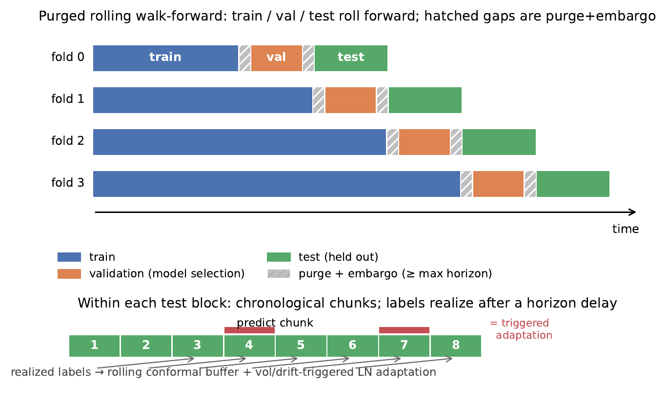
We use strict rolling walk-forward evaluation with chronological separation between train, validation, and test windows. This is the appropriate evaluation design for dependent time series because it respects temporal order and rolling-origin deployment constraints [19, 20]. The exact window lengths may vary by candle scale, but the protocol remains structurally constant: contiguous training data are followed by a validation segment for model selection and a held-out test segment for final reporting, and the entire window then advances forward in time.

Within each held-out test block, the recalibrated-only and adaptive arms are additionally evaluated sequentially: forecasts are issued in chronological chunks; conformal buffers and adaptation triggers consume only labels that have realized by the simulation time, purged by the maximum forecast horizon (the online mirror of the walk-forward embargo); and triggered updates modify the forecaster in place going forward. The static arm uses the same trained model without any within-block updating, so the three arms differ only in their online treatment. Adaptation triggers are causal by construction: the volatility trigger compares the anchor's trailing realized-volatility statistic against a training-split percentile, and the drift trigger compares recent realized pinball loss against the validation baseline.

For the completed reduced study, this rolling protocol is applied independently for each candle granularity on BTCUSDT. Results are then aggregated hierarchically across splits and temporal scales. This makes it possible to distinguish within-asset temporal stability from cross-scale consistency while leaving cross-asset generalization for a later multi-asset pass.

Because the broader family sweep is deferred, the methodology layer freezes a claim-ready benchmark slice before wider comparisons are promoted. This slice keeps the asset scope, horizon family, walk-forward protocol, and artifact schema fixed so that new metrics, ensemble logic, or objective changes can be judged against a stable reference rather than against a moving benchmark definition.

Element	Frozen value
Asset	BTCUSDT USD-M perpetual
Primary scale / horizons	15m, $\{1,4,16\}$ bars
Protocol	purged walk-forward; sequential arms static/conformal/conformal_adapt
Objective	pinball + Huber vol (primary aux) + Huber dd + small direction BCE
Primary readouts	pinball/WQL, coverage error, interval width, vol $R^2$

All results tables in Section 6 are emitted by the report-study pipeline into the runs/report_final_study root and consumed directly by this manuscript; no benchmark ordering is hand-written beyond what those generated tables support. The ten admissible walk-forward variants populate a single aggregated results table (Table 7) whose rows are sample-weighted across folds, so the distinction between contract-only and admissible evidence is carried by the pipeline metadata rather than by editorial assertion.

We report:

• point forecast metrics: MAE and RMSE,
• probabilistic metrics: pinball loss, interval coverage, interval width, and calibration error,
• auxiliary risk-forecast skill: out-of-sample $R^2$ of the volatility and drawdown heads, with volatility skill treated as the primary auxiliary readout given prior evidence on this surface,
• quantile skill scores (QSS): $1 - \text{pinball}_{\text{model}}/\text{pinball}_{\text{marginal}}$ against the training-split unconditional quantiles, reported separately for the return, MFE, and MAE quantile groups — the scan-aligned minimum bar for a quantile forecaster to be meaningful,
• paper-comparability metrics: leak-safe MASE variants, stabilized sMAPE, quantile-approximate CRPS, and weighted quantile loss,
• directional decision metrics: raw directional accuracy, thresholded significant-move directional accuracy, significant-move share, and simple active-signal versus selective-signal signed-return summaries,
• horizon-wise diagnostics: metric summaries stratified by forecast horizon, asset, and task scale.

This metric mix is intentional. Point error alone is insufficient when the model outputs intervals or quantiles; proper probabilistic evaluation also requires scores and diagnostics that measure calibration and sharpness [9, 21]. The maintained decision-relevance contract now treats thresholded directional accuracy as the primary directional readout and uses active-signal and selective-signal summaries only as simple actionability proxies rather than as a full execution backtest. This separation is important because the model is trained with a directional logit loss, not with an accuracy-maximization objective directly, so modest improvements in the optimized directional term may not translate into large gains in raw per-bar hit rate. A model that improves MAE but degrades calibration or directional stability is not actually better for the target application. Conversely, a model with slightly worse point error may still be preferable if it preserves sign quality and produces better calibrated confidence bands. The significant-move threshold is pre-registered rather than searched: a move at horizon $h$ counts as significant when $|r_{T,h}| > \max\bigl(5\ \text{bps},\ \hat\sigma_{T,h}\bigr)$, where $\hat\sigma_{T,h}$ is the trailing causal realized-volatility estimate at the anchor scaled to horizon $h$.

Because the active study spans multiple scales and backbone families on one asset, the final paper should report metrics at three levels: detailed per-split diagnostics, summarized per-scale tables, and pooled comparisons that average over the relevant axes while still exposing variance across them. Where appropriate, paired tests or confidence intervals across rolling splits should be used to distinguish robust gains from noise.

The candidate forecast horizons are no longer restricted to 1, 5, and 15 minutes alone. Instead, horizons are defined relative to each candle granularity so that short, medium, and moderately extended forecasts can be studied at each base scale. The maintained task grids follow the side signal-scale scan's verdicts: $\{1,4,16,96\}$ bars for the fifteen-minute primary task (15 minutes to one day ahead — every cell passes the scan's pre-registered validation-and-test rule for return and excursion quantile skill), $\{1,3,12,288\}$ for the five-minute secondary task, and $\{1,5,15\}$ for the deferred one-minute stress lane. Seven-day horizons failed the scan (quantile skill collapses toward the marginal) and are excluded. The scan also found multiscale fusion gains concentrated at horizons of one day and beyond, which is precisely where the added $h{=}96$ cell sits — sharpening the single-scale-versus-multi-scale ablation.

A representative optimization setup now uses batch size 64, up to 7 epochs per split, learning rate $5 \times 10^{-4}$, weight decay $10^{-4}$, gradient clipping at 1.0, and early stopping with patience 3. The shared report-study baseline assigns nonzero weights to the return-quantile, volatility, drawdown, and (small) directional terms so the maintained benchmark and methodology ablations optimize the same report-goal objective by default; the adaptation-stability penalty applies only during online adaptation updates, as defined in the adaptation section. At the model-config level, the base TimesFM profile remains a pretrained_only and adapter_tune setup with residual bottleneck adapters and split backbone, adapter, and forecasting-head learning rates. The rebuilt benchmark_main_adaptive lane now overrides that base in three linked ways: it switches to small layer_norm_tuning adapters, promotes the main feature surface to the newer temporal-and-freshness-aware exogenous contract, and enables the dual typed-covariate path so future-known calendar and funding-schedule channels can travel beside the maintained flat tensor. Conformal calibration remains enabled with a 64-sample warmup and a 256-sample rolling buffer, implemented as conformalized quantile regression applied jointly to symmetric quantile pairs so that adjustment cannot re-introduce quantile crossing, while online updates stay restricted to layer_norm_only adaptation triggered under high volatility or drift. Beyond the main benchmark, the study contract still separates a methodology-first trustworthy slice, family-specific tuning budgets, calibration ladders, and trainability ladders so optimizer or adaptation choices are not conflated with family identity. Native baseline and transfer evidence are deferred from the active matrix.

The completed study spans eleven walk-forward variants on the BTCUSDT USD-M perpetual surface: a from-scratch multi-resolution benchmark, five pretrained foundation-model lanes (frozen and LoRA-fine-tuned Chronos-T5-small; frozen, attention-LoRA, and capacity-matched expert-LoRA Moirai-MoE-small), four methodology ablations, and a secondary five-minute scale. Every variant is evaluated under the three pre-registered arms (static, conformal recalibration, and conformal-plus-triggered-adaptation) with strict purged walk-forward splits. Table 7 is the authoritative artifact-backed summary emitted by the report-study pipeline; the subsections below interpret it. Skill is reported primarily as the quantile skill score $\mathrm{QSS} = 1 - \text{pinball}_{\text{model}} / \text{pinball}_{\text{marginal}}$ against the training-split unconditional quantiles, for returns and for the two path-excursion targets, alongside the out-of-sample volatility $R^2$ and interval coverage error.

Variant	Arm	QSS$_{ret}$	QSS$_{MFE}$	QSS$_{MAE}$	Vol $R^2$	CovErr	WQL
benchmark_main_15m	static	0.0594	0.1535	0.1552	0.3862	0.0118	0.6707
benchmark_main_15m	conformal	0.0547	0.1535	0.1552	0.3862	0.0048	0.6777
benchmark_main_15m	conformal_adapt	0.0553	0.1565	0.1561	0.3852	0.0055	0.6772
ablation_single_scale_15m	static	0.0579	0.1556	0.1502	0.3741	0.0268	0.6720
ablation_single_scale_15m	conformal	0.0541	0.1556	0.1502	0.3741	0.0051	0.6787
ablation_single_scale_15m	conformal_adapt	0.0543	0.1552	0.1517	0.3769	0.0050	0.6783
ablation_endogenous_only_15m	static	0.0610	0.1497	0.1559	0.3821	0.0232	0.6672
ablation_endogenous_only_15m	conformal	0.0570	0.1497	0.1559	0.3821	0.0048	0.6731
ablation_endogenous_only_15m	conformal_adapt	0.0573	0.1485	0.1524	0.3814	0.0046	0.6729
ablation_no_excursion_supervision_15m	static	0.0574	-0.3770	-0.4813	0.3864	0.0198	0.6715
ablation_no_excursion_supervision_15m	conformal	0.0536	-0.3770	-0.4813	0.3864	0.0054	0.6773
ablation_no_excursion_supervision_15m	conformal_adapt	0.0536	-0.3762	-0.5061	0.3855	0.0053	0.6775
ablation_no_adaptation_15m	static	0.0581	0.1527	0.1531	0.3859	0.0086	0.6710
ablation_no_adaptation_15m	conformal	0.0533	0.1527	0.1531	0.3859	0.0050	0.6779
benchmark_secondary_5m	static	0.0696	0.1670	0.1712	0.4092	0.0100	0.6664
benchmark_secondary_5m	conformal	0.0638	0.1670	0.1712	0.4092	0.0050	0.6776
benchmark_secondary_5m	conformal_adapt	0.0645	0.1668	0.1713	0.4062	0.0051	0.6763
chronos_frozen_15m	static	0.0430	0.1422	0.1395	0.3664	0.0270	0.6957
chronos_frozen_15m	conformal	0.0399	0.1422	0.1395	0.3664	0.0051	0.7008
chronos_frozen_15m	conformal_adapt	0.0415	0.1446	0.1403	0.3690	0.0047	0.6987
chronos_finetune_lora_15m	static	0.0558	0.1460	0.1435	0.3709	0.0159	0.6752
chronos_finetune_lora_15m	conformal	0.0516	0.1460	0.1435	0.3709	0.0042	0.6819
chronos_finetune_lora_15m	conformal_adapt	0.0521	0.1481	0.1441	0.3729	0.0042	0.6814
moirai_frozen_15m	static	0.0584	0.1456	0.1485	0.3686	0.0137	0.6682
moirai_frozen_15m	conformal	0.0536	0.1456	0.1485	0.3686	0.0051	0.6751
moirai_frozen_15m	conformal_adapt	0.0537	0.1461	0.1482	0.3688	0.0050	0.6750
moirai_finetune_lora_15m	static	0.0561	0.1455	0.1483	0.3627	0.0119	0.6708
moirai_finetune_lora_15m	conformal	0.0511	0.1455	0.1483	0.3627	0.0049	0.6781
moirai_finetune_lora_15m	conformal_adapt	0.0513	0.1453	0.1486	0.3632	0.0050	0.6782
moirai_finetune_expert_lora_15m	static	0.0538	0.1408	0.1410	0.3576	0.0159	0.6726
moirai_finetune_expert_lora_15m	conformal	0.0487	0.1408	0.1410	0.3576	0.0051	0.6799
moirai_finetune_expert_lora_15m	conformal_adapt	0.0489	0.1410	0.1416	0.3587	0.0054	0.6795

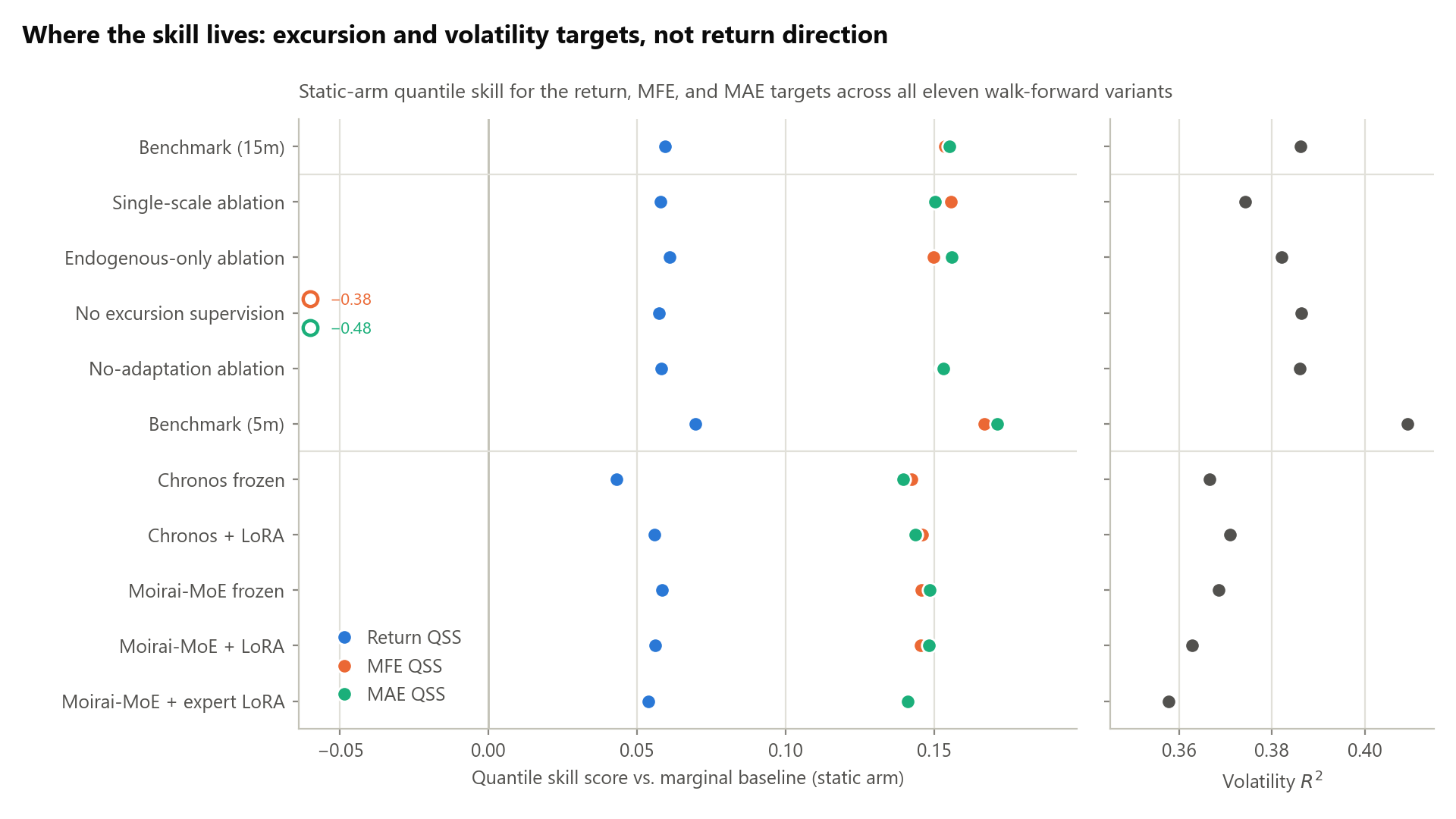
The predictable structure on this surface is distributional and concentrated in the path-excursion and volatility targets, not in the direction of the return. The benchmark model attains quantile skill of $+0.153$ (maximum favorable excursion) and $+0.155$ (maximum adverse excursion) over the unconditional baseline, a volatility $R^2$ of $0.386$, and a smaller but positive return-quantile skill of $+0.059$. That the excursion skill is genuine conditional structure rather than an artifact of the head is confirmed by the excursion-supervision ablation: removing the excursion loss terms collapses their quantile skill to $-0.377$ and $-0.481$ (worse than the marginal, as expected for untrained heads) while leaving return-quantile skill essentially unchanged ($+0.057$ vs $+0.059$). Excursion supervision therefore adds a strong, decision-relevant readout at no cost to the return fit. This matches the pre-registered signal-scale scan that motivated promoting the excursion quantiles to first-class targets, and it is the property the downstream order-placement layer consumes: take-profit and stop-loss levels are read directly from the conditional MFE and MAE quantiles.

The central comparative result is that no pretrained foundation-model lane, frozen or fine-tuned, beats the two-million-parameter from-scratch multi-resolution encoder on any distributional metric. On the static arm the scratch benchmark leads on return-quantile skill ($+0.059$), both excursion skills ($+0.153$, $+0.155$), and volatility $R^2$ ($0.386$); every foundation-model variant ties or trails. Given that the scratch encoder is roughly an order of magnitude smaller than the smallest foundation models considered and is trained end-to-end on the same windows, it is the quality-versus-cost frontier for this task.

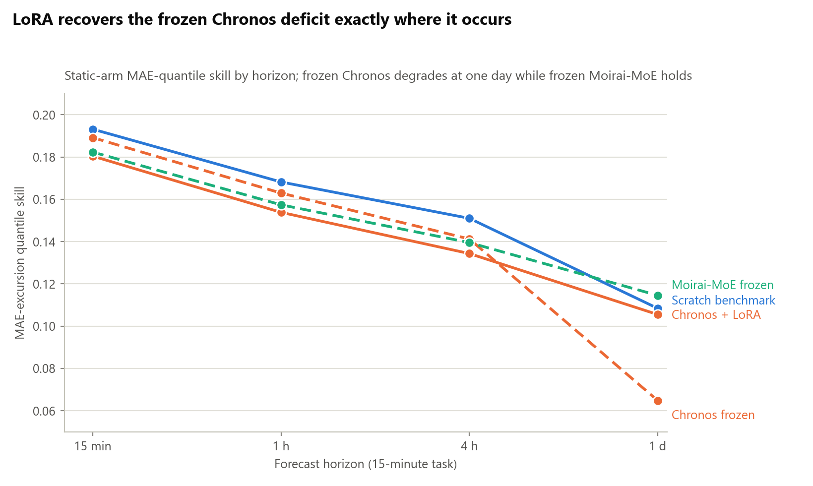
The families differ markedly in the quality of their frozen representations, however, and this is the finding most relevant to downstream Moirai-MoE work. The frozen Moirai-MoE representation is competitive with the scratch encoder ($+0.058$ return-quantile skill, $0.369$ volatility $R^2$) and clearly stronger than the frozen Chronos representation ($+0.043$, $0.366$). The gap is sharpest at the one-day horizon, where frozen Chronos degrades to an MAE-quantile skill of $+0.065$ while frozen Moirai holds at $+0.115$, matching or exceeding the scratch encoder's $+0.108$. In other words, a frozen Moirai-MoE encoder already carries most of the usable distributional structure on this surface without any adaptation, whereas a frozen Chronos encoder does not, particularly at longer horizons.

LoRA fine-tuning recovers a frozen representation where it is deficient but cannot improve one that is already strong—and where there is no deficit to recover, it slightly degrades the representation. For Chronos, rank-8 LoRA on the attention query/value projections lifts return-quantile skill from $+0.043$ to $+0.056$ and, most tellingly, restores the one-day MAE-quantile skill from $+0.065$ to $+0.106$—almost fully closing the frozen model's horizon-specific deficit and bringing it in line with the scratch benchmark. For Moirai, whose frozen representation is already competitive with the scratch encoder, fine-tuning does not help under either of two adaptations of increasing capacity. The same attention-only LoRA is inert (return-quantile skill $+0.058 \rightarrow +0.056$). A capacity-matched expert LoRA that additionally adapts every mixture-of-experts projection—fc1, fc2, and fc_gate across all thirty-two experts and six layers, about $4.5$ million trainable parameters or roughly twenty times the attention-only adapter, with routing frozen—does not recover the null and in fact mildly underperforms the frozen model on every distributional metric (return-quantile skill $+0.058 \rightarrow +0.054$; MAE-quantile skill $+0.148 \rightarrow +0.141$; volatility $R^2$ $0.369 \rightarrow 0.358$), with the small degradation concentrated at the shortest horizons. This resolves the earlier ambiguity: the inertness of Moirai fine-tuning is not an adapter-capacity artifact—reaching the experts, where $97\%$ of the model's parameters live, does not help either. The clean reading across both families is that the value of fine-tuning a foundation-model backbone is a direct function of how deficient its frozen representation is on the target surface. Chronos begins with a recoverable deficit and adaptation closes it; Moirai begins near the representational ceiling for this task, so adapting it on the limited single-asset data only perturbs a good representation.

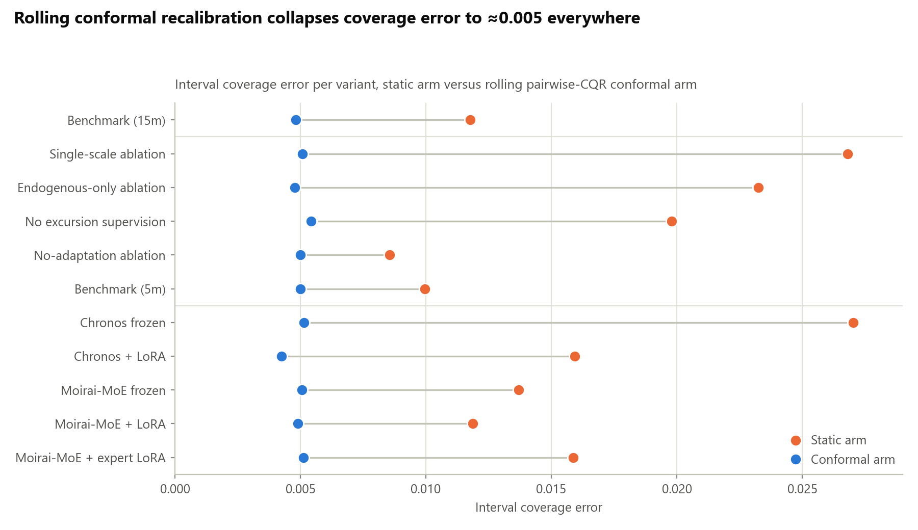
Interval calibration is solved by the rolling pairwise-CQR recalibration arm across every variant. Static-arm coverage error ranges from $0.009$ to $0.027$ (the foundation-model lanes are the least well calibrated out of the box, e.g. frozen Chronos at $0.027$), and the conformal arm collapses all of them to approximately $0.005$ without measurably degrading the point or excursion skills. Because the recalibration is applied to symmetric quantile pairs with outward re-monotonization, it never reintroduces quantile crossing. Calibration is therefore not a differentiator between models on this surface: it is a post-hoc guarantee that the conformal layer supplies uniformly.

The methodology ablations are, with one exception, null or small. Removing the exogenous branch (funding, basis, calendar) does not degrade skill—the endogenous-only variant is statistically indistinguishable from the full benchmark and marginally higher on return-quantile skill ($+0.061$ vs $+0.059$)—indicating that the engineered derivatives-state features add no measurable distributional skill at these scales. Reducing the input to a single temporal resolution costs little in aggregate ($0.386 \rightarrow 0.374$ volatility $R^2$; return-quantile skill essentially unchanged), and the small multi-resolution gain that does exist is concentrated at the one-day horizon, consistent with the scan's prediction that cross-scale context matters most at longer horizons. Triggered online adaptation is effectively inert: the conformal-plus-adaptation arm is indistinguishable from conformal-only on every variant, so the value in the sequential pipeline comes entirely from recalibration rather than from parameter adaptation. Only the excursion-supervision ablation of Section 6.1 moves the headline metrics, and it does so by design.

Moving the base task from fifteen-minute to five-minute candles improves every distributional metric: the five-minute benchmark attains the study's best return-quantile skill ($+0.070$), excursion skills ($+0.167$, $+0.171$), and volatility $R^2$ ($0.409$). The finer scale exposes more conditional structure rather than more noise, which is consistent with the signal-scale scan finding that skill is strongest at fine granularities and decays with physical horizon. This identifies the finer scales, together with the excursion and volatility targets, as the most promising surface for the order-placement application.

The proposed framework is motivated by three core ideas: that short-horizon financial dynamics are strongly scale dependent, that uncertainty should be modeled explicitly rather than indirectly, and that non-stationary environments require some form of adaptation or recalibration. These principles are conceptually well aligned with the stylized facts of cryptocurrency markets, but their practical value must be established through careful rolling evaluation rather than architectural intuition alone.

Several limitations should therefore be stated directly. The study is single-asset and single-family-size: it compares the larger maintained Chronos-T5-small and Moirai-MoE-small checkpoints on BTCUSDT only, and within-family size scaling, native-decoder baselines, and cross-asset transfer are deferred. The fine-tuning evidence spans two adaptation capacities per family—attention-only LoRA and, for Moirai, a capacity-matched expert LoRA reaching the mixture-of-experts blocks—but leaves the model routing frozen and does not attempt a full unfreeze; the negative Moirai fine-tuning result should be read within those bounds, though the fact that it holds even when the experts are adapted makes an adapter-capacity explanation unlikely. The empirical finding on exogenous variables is a concrete instance of a general caution: the engineered funding, basis, and calendar features added no measurable distributional skill on this surface, confirming that the usefulness of exogenous signals depends on their causal alignment and regime-specific informativeness rather than on their inclusion alone.

More broadly, the framework may generalize to other financial or non-financial systems that share the same basic properties of nonlinear dynamics, incomplete observation, and persistent distribution shift. Within the present scope, the decisive comparison has been run: across four foundation-model lanes and a from-scratch encoder on a tractable BTCUSDT matrix, the smallest model is the quality-versus-cost frontier, the value of a pretrained backbone is entirely in the quality of its frozen representation and in whether fine-tuning can recover a deficit, and the usable signal is distributional and excursion-dominated. The trustworthy-slice governance, paper-comparability metrics, and family-faithfulness checks make these findings interpretable as more than a single-number leaderboard.

This paper presents a regime-adaptive probabilistic forecasting framework for short-horizon cryptocurrency prediction and organizes it as a clear experimental study. The central idea is to combine multi-resolution temporal encoding, engineered exogenous market conditioning, probabilistic forecasting, and lightweight adaptation within a chronologically valid evaluation design. Rather than emphasizing implementation logistics, the paper focuses on the hypotheses, data design, baselines, metrics, trust-building slices, and interpretation rules needed for a defensible empirical assessment.

The completed matrix supports a clear set of conclusions and points to specific next steps. Empirically, on the BTCUSDT surface the from-scratch multi-resolution encoder is the quality-versus-cost frontier; a frozen Moirai-MoE representation is competitive with it while a frozen Chronos representation is not; LoRA fine-tuning recovers the Chronos deficit precisely where it occurs but neither attention nor capacity-matched expert adaptation improves the already-strong Moirai representation; rolling conformal recalibration supplies uniform interval calibration; and the usable structure lives in the excursion and volatility quantiles at finer temporal scales. The natural extensions follow directly from the study's scope boundaries: within-family size scaling, a full (rather than low-rank, routing-frozen) fine-tune to probe the ceiling of backbone adaptation, and a multi-asset pass to test whether the excursion-and-volatility signal and the family ordering transfer beyond BTCUSDT [19, 20, 22].

Optional acknowledgments here.

The study is organized around three interacting design choices:

• Temporal resolution: comparison between single-scale and multi-scale input representations.
• Information set: comparison between endogenous-only inputs and models augmented with causally aligned exogenous variables.
• Adaptation strategy: comparison between static models, calibrated models, and lightweight regime-adaptive variants.

These factors define the main ablation surface of the experiment.

References

- R. Cont. Empirical properties of asset returns: Stylized facts and statistical issues. Quantitative Finance, 2001. https://www.researchgate.net/publication/313727065_Empirical_properties_of_asset_returns_Stylized_facts_and_statistical_issues
- A. W. Lo. The adaptive markets hypothesis: Market efficiency from an evolutionary perspective. Journal of Portfolio Management, 2004. https://web.mit.edu/Alo/www/Papers/JPM2004.html
- M. O'Hara. Market microstructure. In Handbook of the Economics of Finance, 2003. https://www.sciencedirect.com/science/chapter/handbook/pii/S1574010203010136
- P. Katsiampa. Volatility estimation for Bitcoin: A comparison of GARCH models. Economics Letters, 2017. https://www.sciencedirect.com/science/article/pii/S0165176517302501
- Regime changes in Bitcoin GARCH volatility dynamics. Finance Research Letters, 2019. https://www.sciencedirect.com/science/article/pii/S1544612318303970
- Stylized facts of cryptocurrency markets: Similarities and differences to conventional markets. 2026. https://www.sciencedirect.com/science/article/pii/S156601412600004X
- Regime-switching in Bitcoin volatility. Research in International Business and Finance, 2026. https://www.sciencedirect.com/science/article/pii/S027553192600022X
- V. Flunkert, D. Salinas, and J. Gasthaus. DeepAR: Probabilistic forecasting with autoregressive recurrent networks. 2017. https://www.researchgate.net/publication/316098318_DeepAR_Probabilistic_Forecasting_with_Autoregressive_Recurrent_Networks
- T. Gneiting and A. E. Raftery. Strictly proper scoring rules, prediction, and estimation. Journal of the American Statistical Association, 2007. https://colab.ws/articles/10.1198%2F016214506000001437
- R. Koenker and G. Bassett. Regression quantiles. Econometrica, 1978. https://econpapers.repec.org/article/ecmemetrp/v_3a46_3ay_3a1978_3ai_3a1_3ap_3a33-50.htm
- B. Lim, S. Arik, N. Loeff, and T. Pfister. Temporal fusion transformers for interpretable multi-horizon time series forecasting. International Journal of Forecasting, 2021. https://research.google/pubs/temporal-fusion-transformers-for-interpretable-multi-horizon-time-series-forecasting/
- A time series is worth 64 words: Long-term forecasting with transformers. ICLR, 2023. https://iclr.cc/virtual/2023/poster/10876
- Neural basis expansion analysis with exogenous variables: Forecasting with NBEATSx. 2023. https://www.sciencedirect.com/science/article/pii/S0169207022000413
- J. Gama, I. Zliobaite, A. Bifet, M. Pechenizkiy, and A. Bouchachia. A survey on concept drift adaptation. ACM Computing Surveys, 2014. http://repositorio.inesctec.pt/handle/123456789/5370
- E. J. Hu et al. LoRA: Low-rank adaptation of large language models. 2021. https://arxiv.gg/abs/2106.09685
- Deribit Support. Inverse perpetual. Updated January 21, 2026. https://support.deribit.com/hc/en-us/articles/31424954847133-Inverse-Perpetual
- Reconciling open interest with traded volume in perpetual swaps. Ledger, 2024. https://ledgerjournal.org/ojs/ledger/article/view/325
- CME Group. Open interest. https://www.cmegroup.com/education/courses/introduction-to-futures/open-interest
- L. J. Tashman. Out-of-sample tests of forecasting accuracy: An analysis and review. International Journal of Forecasting, 2000. https://www.sciencedirect.com/science/article/pii/S0169207000000650
- C. Bergmeir and J. M. Benitez. On the use of cross-validation for time series predictor evaluation. Information Sciences, 2012. https://www.sciencedirect.com/science/article/pii/S0020025511006773
- J. Brocker and L. A. Smith. Increasing the reliability of reliability diagrams. Weather and Forecasting, 2007. https://www.researchgate.net/publication/228534099_Increasing_the_Reliability_of_Reliability_Diagrams
- D. H. Bailey, J. M. Borwein, M. Lopez de Prado, and Q. J. Zhu. Pseudo-mathematics and financial charlatanism: The effects of backtest overfitting on out-of-sample performance. Notices of the AMS, 2014. https://papers.ssrn.com/sol3/papers.cfm?abstract_id=2308659
A. Additional Experimental Details