Where Is the Signal? A Scale Scan of BTCUSDT Perpetual Futures for Distributional Forecasting
Side study feeding the regime-adaptive forecasting programme
Abstract
Before committing a multi-backbone forecasting study to a particular timeframe and target family, we ask the prior question directly: at which temporal scales, horizons, and target definitions does the BTCUSDT USD-M perpetual series carry learnable signal at all? We scan the full canonical store (1 m–1 d bars, 2019–2026) with small standardized probes under a strict chronological purged protocol, measuring four things per (timeframe, horizon) cell: quantile skill of conditional return distributions over the unconditional (marginal) baseline; out-of-sample $R^2$ on log realized volatility; directional discriminability; and — the decision-relevant novelty — quantile skill on forward path extremes (maximum favorable and adverse excursion computed from high/low prices), which are precisely the quantities take-profit and stop-loss placement requires. A multiscale fusion probe tests whether coarser-timeframe context adds skill at a fixed base scale. Verdicts against pre-registered thresholds, required to hold on both validation and test, determine where the main study's backbone comparison will be pointed. The scan is deliberately model-light: the question is whether any conditioning beats the marginal distribution at a scale, not which architecture does so best.
1. Motivation
The parent project (Regime-Adaptive Probabilistic Foundation Models…) compares pretrained sequence-model families under a common probabilistic head on BTCUSDT. Prior internal evidence on this surface is sobering: at 15 m–3 d horizons, direction is not predictable to a cost-surviving degree from either frozen foundation-model embeddings or causal bar features (out-of-sample directional accuracy $\approx 0.50$), while conditional volatility is strongly predictable (test $R^2 \approx 0.40$ at 4 h). A backbone comparison run on a signal-free cell of the (scale, horizon, target) space measures only noise. This study therefore maps the space first, so that the comparison is staged where a detectable signal exists, and so that the final model's outputs are the distributional quantities an execution layer can consume directly.
Decision relevance. The intended consumer places market orders with attached take-profit and stop-loss levels. The distributional objects that matter for that decision are not only the terminal return $r_{T,h}$ but the path extremes over the holding window: how far price travels in one's favor (governs achievable take-profit) and against (governs stop placement and survival). Both are computed here from high/low prices, not close-to-close approximations.
2. Data
All series come from the repository's canonical Binance USD-M perpetual store (binance_usdm/btcusdt), full history 2019-09 to 2026-06: 1 m (3.54 M bars), 5 m (708 k), 15 m (236 k), 1 h (59 k), 4 h (14.7 k), and 1 d (2.5 k), each with OHLCV and an as-of funding-rate series (joined backward with a 16 h staleness tolerance; missing stretches are mask-gated, never imputed). Timeframes are consumed at their native store granularity. Horizon grids overlap in physical time across timeframes (a 4 h-ahead target is reachable from 1 m, 5 m, 15 m, and 1 h representations), so representation scale can be compared at fixed physical horizon.
3. Targets
For anchor bar $T$ and horizon $h$ (bars), with log close $p_t$, log high $g_t$, log low $\ell_t$, and one-bar log returns $r_t$:
Conditional quantiles of $\mathrm{MFE}$ and $\mathrm{MAE}$ are the direct inputs to take-profit and stop-loss placement: e.g. a stop at the conditional 95th percentile of $\mathrm{MAE}$ bounds the probability of being stopped out by path noise.
4. Probes and skill metrics
Features are strictly causal per timeframe: past returns over $\{1,\dots,64\}$-bar lags, trailing volatilities, volume and range $z$-scores, funding (mask-gated), and calendar sin/cos. Probes are small two-layer MLPs (monotone quantile head for distributional targets; regression and logistic heads otherwise), standardized on the training split, early-stopped on validation. The deliberate smallness is the point: we test for the existence of conditional structure, not for architectural superiority.
Skills per cell:
- QSS (quantile skill score) $= 1 - \text{pinball}_{\text{model}} / \text{pinball}_{\text{marginal}}$, where the marginal baseline predicts the training split's unconditional quantiles. $\mathrm{QSS} > 0$ is the minimum bar for a quantile forecaster to be meaningful at all. Applied to returns, MFE, MAE.
- vol $R^2$: out-of-sample $R^2$ on $y^{\text{vol}}$ against the train-mean baseline.
- dir AUC / accuracy: rank AUC of a directional logit.
Protocol. Chronological 70/10/20 split per timeframe with a purge of $\lceil h_{\max}/\text{stride} \rceil$ anchors at each boundary. Pre-registered verdict rule: a cell has signal only if the skill clears its threshold ($\mathrm{QSS} > 0.02$; vol $R^2 > 0.05$; AUC $> 0.52$) on both validation and test. Requiring agreement guards against the non-stationary flukes observed in earlier internal studies (validation edges that vanish on test).
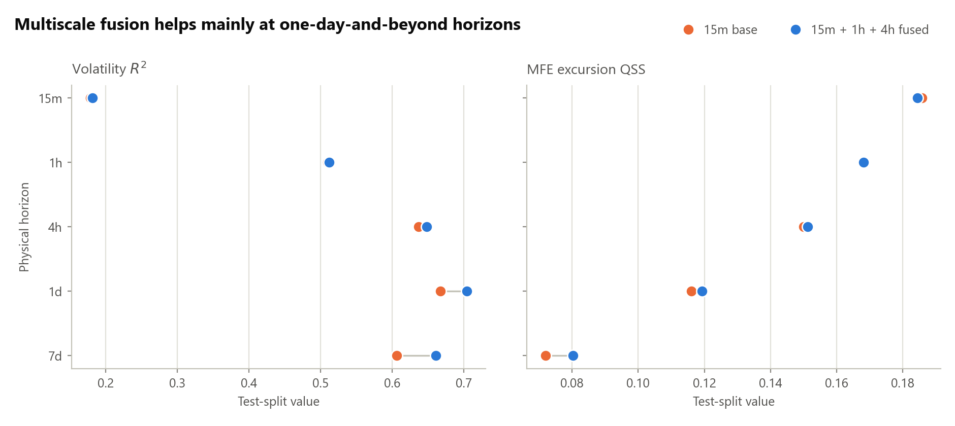
Multiscale fusion. For a base timeframe, features from coarser timeframes are appended after leak-safe alignment: a coarser bar's features become available only at that bar's close (joining on bar-start timestamps would leak the still-open bar). The change in QSS / $R^2$ relative to the base-only cell measures the value of multiscale input — directly informing the parent study's multi-resolution design.
5. Results
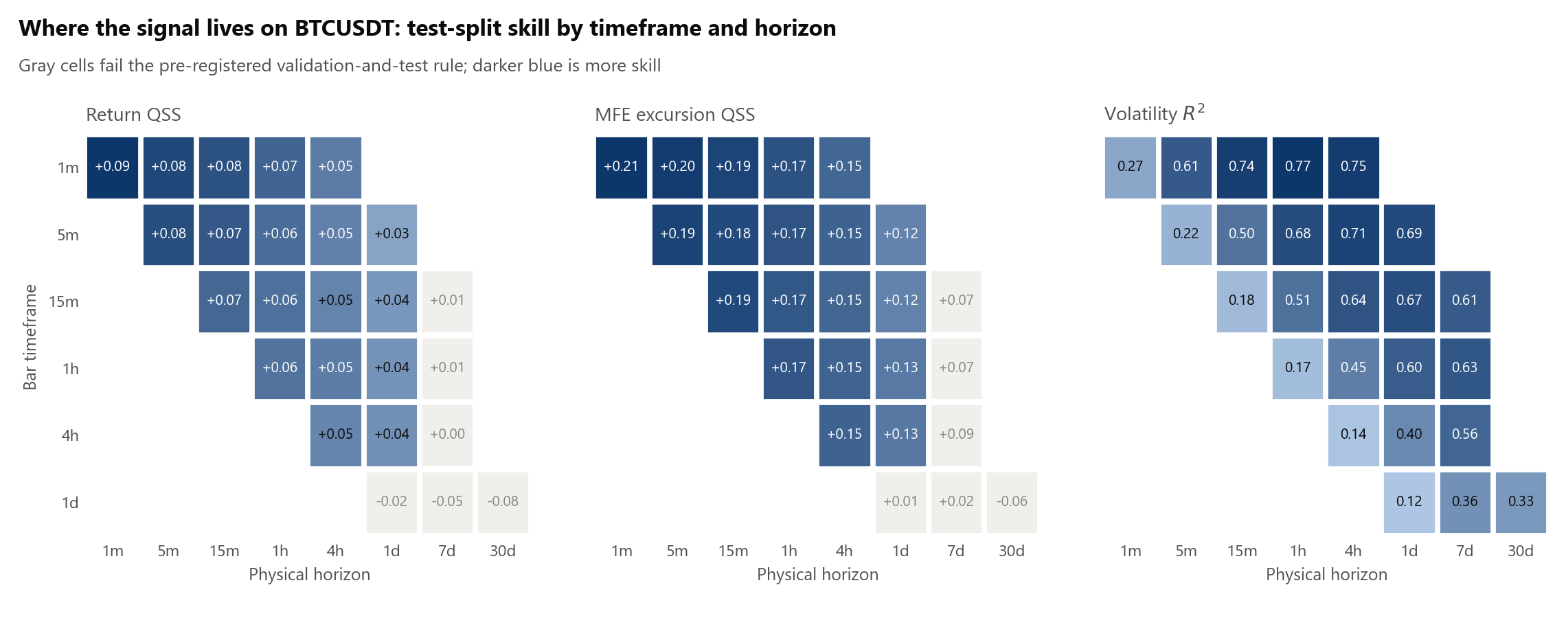
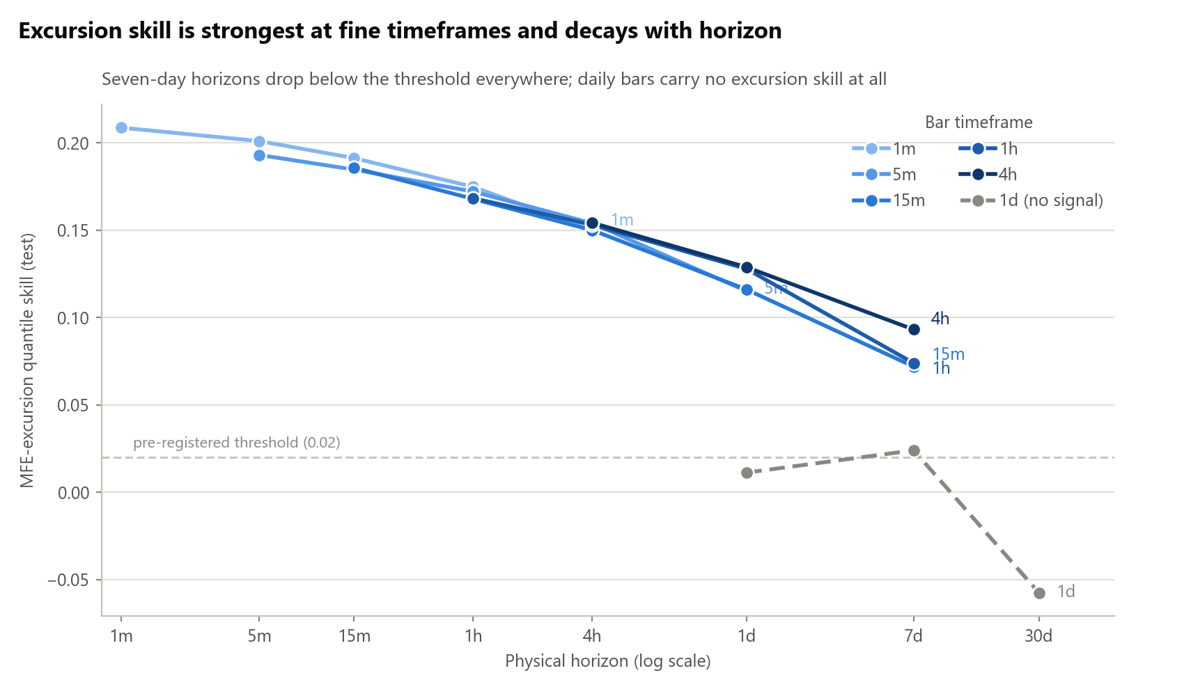
Generated by python -m sss scan --config configs/scan.yaml; the table below is produced by the scan pipeline (bold cells pass the pre-registered rule on validation and test jointly).
| TF | Horizon | QSS$_{ret}$ | vol $R^2$ | dir AUC | QSS$_{MFE}$ | QSS$_{MAE}$ | $n_{test}$ |
|---|---|---|---|---|---|---|---|
| 1m | 1m | +0.092 | +0.269 | +0.524 | +0.209 | +0.205 | 44218 |
| 1m | 5m | +0.082 | +0.611 | +0.522 | +0.201 | +0.194 | 44218 |
| 1m | 15m | +0.077 | +0.739 | +0.530 | +0.191 | +0.191 | 44218 |
| 1m | 1h | +0.067 | +0.773 | +0.522 | +0.175 | +0.174 | 44218 |
| 1m | 4h | +0.054 | +0.746 | +0.519 | +0.150 | +0.152 | 44218 |
| 5m | 5m | +0.079 | +0.216 | +0.520 | +0.193 | +0.189 | 35304 |
| 5m | 15m | +0.073 | +0.500 | +0.531 | +0.185 | +0.186 | 35304 |
| 5m | 1h | +0.063 | +0.677 | +0.529 | +0.172 | +0.167 | 35304 |
| 5m | 4h | +0.051 | +0.715 | +0.527 | +0.154 | +0.149 | 35304 |
| 5m | 1d | +0.033 | +0.690 | +0.524 | +0.115 | +0.101 | 35304 |
| 15m | 15m | +0.065 | +0.179 | +0.542 | +0.186 | +0.173 | 23178 |
| 15m | 1h | +0.061 | +0.510 | +0.532 | +0.168 | +0.165 | 23178 |
| 15m | 4h | +0.050 | +0.637 | +0.530 | +0.150 | +0.148 | 23178 |
| 15m | 1d | +0.040 | +0.667 | +0.532 | +0.116 | +0.107 | 23178 |
| 15m | 7d | +0.008 | +0.606 | +0.520 | +0.072 | +0.073 | 23178 |
| 1h | 1h | +0.059 | +0.167 | +0.535 | +0.168 | +0.161 | 11573 |
| 1h | 4h | +0.054 | +0.448 | +0.531 | +0.153 | +0.145 | 11573 |
| 1h | 1d | +0.042 | +0.601 | +0.532 | +0.128 | +0.114 | 11573 |
| 1h | 7d | +0.014 | +0.627 | +0.535 | +0.074 | +0.067 | 11573 |
| 4h | 4h | +0.049 | +0.135 | +0.525 | +0.154 | +0.150 | 2875 |
| 4h | 1d | +0.043 | +0.398 | +0.529 | +0.129 | +0.110 | 2875 |
| 4h | 7d | +0.001 | +0.558 | +0.527 | +0.093 | +0.055 | 2875 |
| 1d | 1d | -0.021 | +0.125 | +0.524 | +0.011 | +0.105 | 431 |
| 1d | 7d | -0.049 | +0.364 | +0.491 | +0.024 | +0.049 | 431 |
| 1d | 30d | -0.077 | +0.332 | +0.444 | -0.057 | -0.063 | 431 |
| 15m+1h+4h | 15m | +0.063 | +0.182 | +0.535 | +0.184 | +0.171 | 23178 |
| 15m+1h+4h | 1h | +0.061 | +0.512 | +0.528 | +0.168 | +0.165 | 23178 |
| 15m+1h+4h | 4h | +0.051 | +0.648 | +0.528 | +0.151 | +0.152 | 23178 |
| 15m+1h+4h | 1d | +0.043 | +0.704 | +0.530 | +0.119 | +0.117 | 23178 |
| 15m+1h+4h | 7d | +0.016 | +0.661 | +0.529 | +0.080 | +0.057 | 23178 |
6. Interpretation and pivot rules
The scan's verdicts pivot the parent study as follows:
- Target family. Backbone comparison is staged on the target families that show signal (expected, from prior evidence: volatility and excursion/return quantiles, not direction). Directional metrics remain diagnostics.
- Scale and horizon. The primary benchmark cell moves to the (timeframe, horizon) region with the strongest, val/test-consistent QSS — including the excursion targets, since those feed order placement.
- Multiscale. If the fusion deltas are positive, the multi-resolution encoder keeps its multi-scale views and the paper's ablation gains a cross-timeframe fusion arm; if they are flat, the multi-resolution claim is narrowed accordingly.
- Execution layer. The final model's contract is fixed to emit conditional quantiles of $(y^{\text{ret}}, \mathrm{MFE}, \mathrm{MAE})$ per horizon, from which take-profit / stop-loss / entry filters are derived mechanically.
Reproducibility
One command per artifact: the scan (sss scan), this document's results table (emitted by the scan), and the synthetic self-validation (pytest signal_scale_scan/tests) in which a generator with persistent volatility and coin-flip direction must yield vol/quantile signal and no directional signal. All thresholds above were fixed before the real data was scanned.