Proposals for a Cryptocurrency Trading AI

Wavelets and Generative Adversarial Networks for Extrapolating Random Signals

Abstract

This is the founding concept paper for a multi-year line of work on wavelet-conditioned generative models for short-horizon Bitcoin forecasting. It argues that although Bitcoin's price behaves like a random walk, its minute-to-minute changes hold a near-invariant, zero-mean distribution that a learning system can exploit. From that premise it sketches a complete trading system — an exchange interface, a wavelet-and-GAN prediction model, and a profit-seeking decision layer — and is explicit about where the idea is promising and where it is unproven. The rigorous architecture and the experiments that test it are taken up in the later parts of this series.

This page is intentionally a proposal. It establishes the motivation, the empirical premise, and the system design at a conceptual level. The full generator and discriminator architecture, loss construction, and held-out evaluation are documented in the Wavelet GAN Trading Prototype, and the first end-to-end MATLAB experiment is the WaveGAN BTCUSDT Extrapolation Report. To avoid repeating that material, the architecture sections here stay at the level of intent and rationale.

Introduction

Since the advent of Bitcoin in 2009, decentralized cryptocurrencies have become a fixture of financial discussion. Their growth is uncharacteristic of an ordinary emerging market, and their persistence is unlike that of a typical bubble. Part of the fascination is practical: when compared with other assets, cryptocurrency prices are highly volatile and notoriously difficult to forecast. A strategy that looks profitable one week — trading on a relative-strength signal, say — can reverse and lose money days later.

Beneath that volatility, however, sits a stable statistic. The change in price from one observation to the next — here, the minute-to-minute change in close price — keeps a remarkably consistent distribution that is largely independent of time or market regime. Two equally sized samples drawn at very different times look alike once viewed without reference to absolute price, and that regularity extends, to a degree, into the spectral content of those samples.

The proposal that follows is an AI that exploits the similarity in the frequency content of nearby samples to make useful short-horizon predictions and, from them, profitable trades. Recent behaviour is exposed through a complex wavelet transform before a neural network produces a forecast. Crucially, the network is trained adversarially: rather than chasing a single precise number, it learns to reproduce the stochasticity of the signal shifted forward in time. For live trading, a plausible distribution of futures is more useful than a brittle point estimate.

Several safeguards run throughout the system to blunt the effect of noisy, fundamentally chaotic data: robust statistics, low-pass filtering, and redundant reweighted predictions. The result performs decently in a simulated trading environment. The input, prediction, and output layers are working components; the prediction layer is functional if not fully optimized, and several decision layers are proposed.

One caution is stated plainly. The decision to deploy this for real money is outside the scope of this paper and is not recommended on the basis of these results. The simulator does not model market impact, so its outcomes do not transfer to a live setting, and a system like this would most likely lose money without substantial further work. What matters here is the underlying observation: a seemingly random signal can carry constant properties that a wavelet-equipped, adversarially trained network can use to predict.

Concept

The system is empirically grounded and, by design, robust to lapses in human judgement. It does, however, rest on a few assumptions about how cryptocurrency prices behave — chiefly assumptions about their fundamental randomness — and those assumptions shape every later decision.

A random walk with an invariant increment

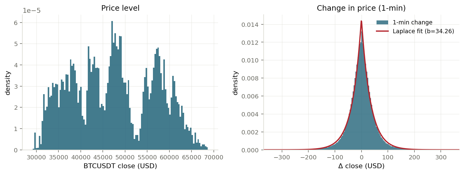
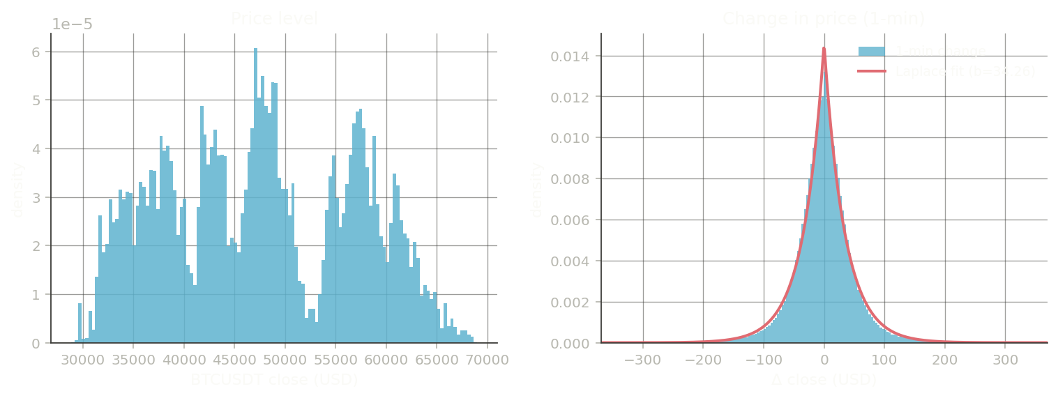
At a glance the price of Bitcoin looks like a random walk: a histogram of one-minute close prices across roughly a year of data shows no stationary structure, and the level wanders without settling on any characteristic value. The distribution of one-minute changes is a different story. It is sharply peaked at zero, approximately symmetric, and close to a Laplace distribution — and it stays that way through time.

Left: broad multi-modal distribution of BTCUSDT one-minute close prices. Right: sharply peaked, near-zero-mean distribution of one-minute price changes with a fitted Laplace curve. — About a year of one-minute BTCUSDT candles (525,906 candles, March 2021–March 2022). The price level has no stationary distribution (left), while the one-minute change is tightly peaked, near zero-mean, and well described by a Laplace fit (right).

$$ \mathcal{B}(t) \left \{ t,\mathcal{B}(t) \in \mathbb{R} : t,\mathcal{B}(t) > 0 \right \} $$

Where $\mathcal{B}$ denotes the price of Bitcoin at an arbitrary time $t$.

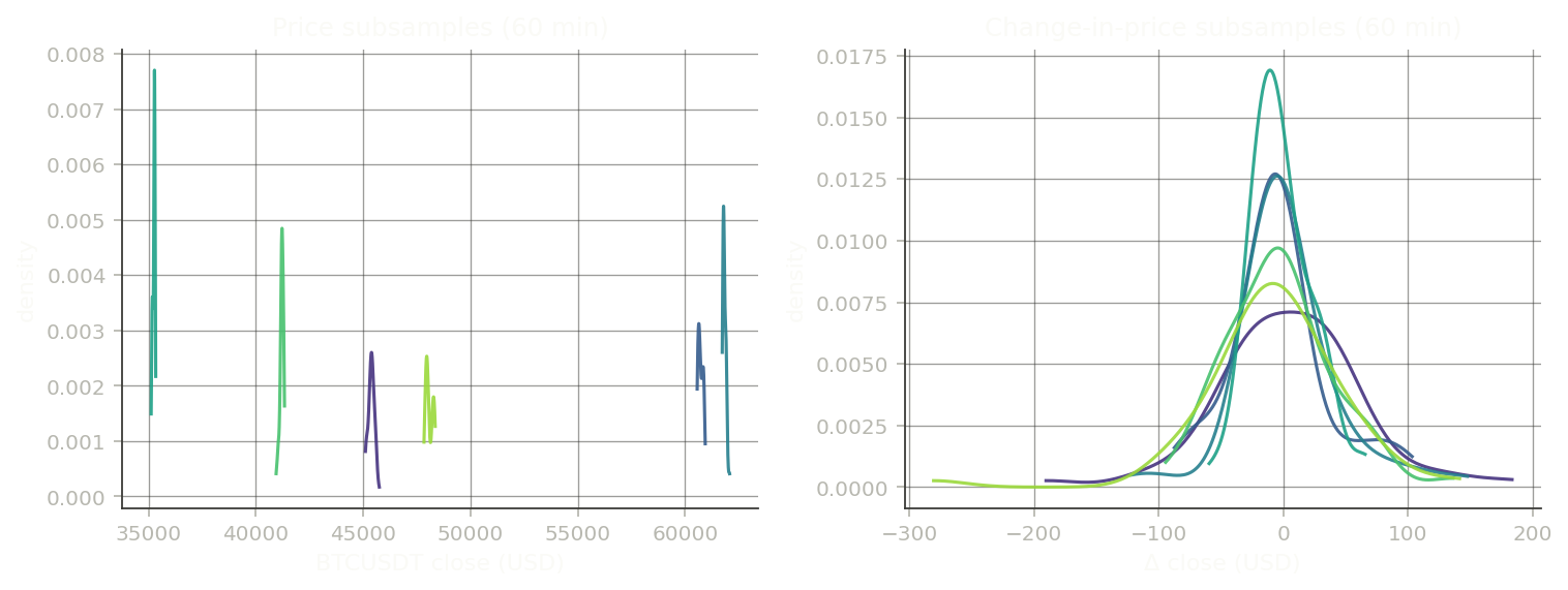
The regularity is not only global. Subsamples drawn from the change-in-price series resemble one another and the parent distribution, with similar means and variances; subsamples drawn from the price series do not. Sixty-minute windows of the change cluster near zero mean with comparable spread, while sixty-minute windows of price sit at disjoint levels that reflect wherever the market happened to be.

$$ \mathbb{E}\left [ \mathcal{B}'(_{n}^{n+w_s}) \right ] \approx \mathbb{E}\left [ \mathcal{B}'(_{m}^{m+w_s}) \right ] $$

For arbitrary times $m$ and $n$, and sample window size $w_s$.

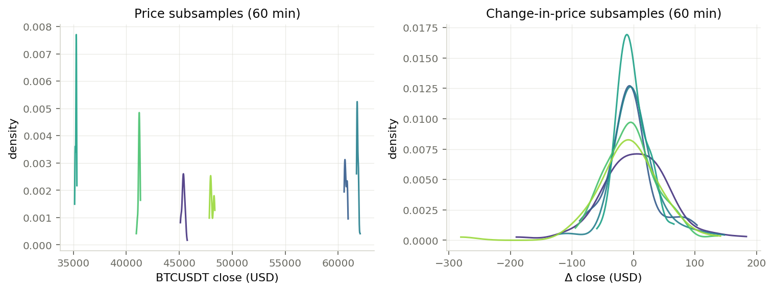
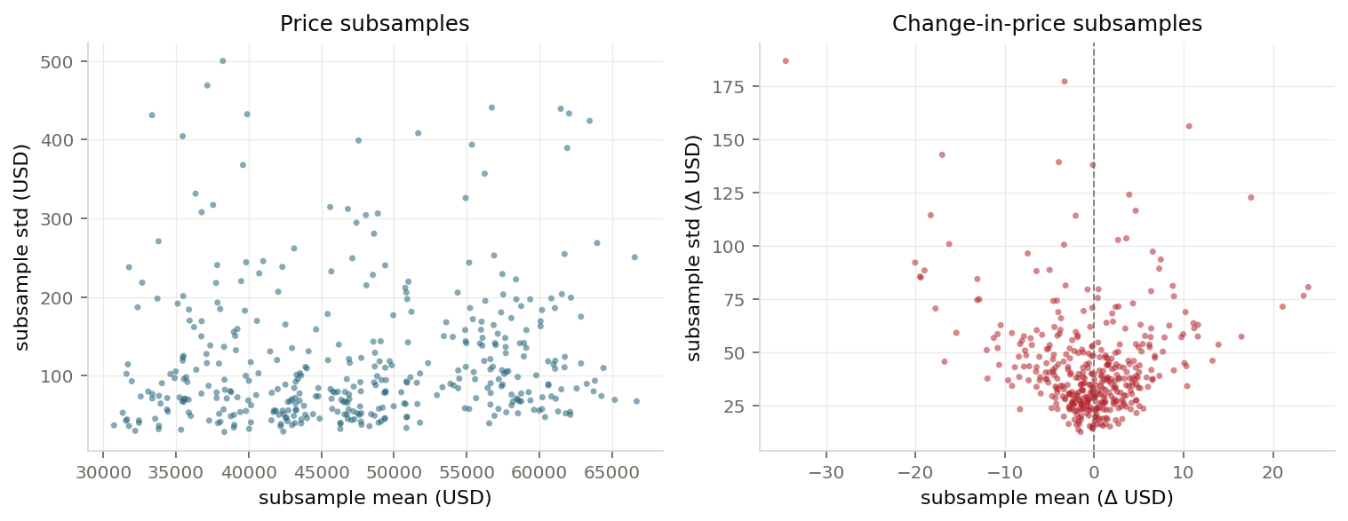
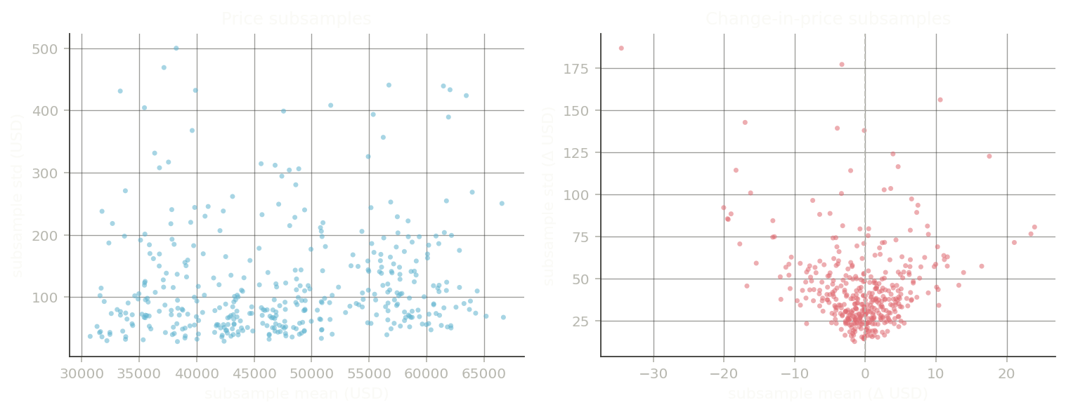
Density curves for several 60-minute subsamples. Price subsamples occupy disjoint narrow ranges; change-in-price subsamples overlap near zero with similar shapes. — Six random sixty-minute subsamples. Price subsamples (left) are narrow and sit at unrelated levels; change-in-price subsamples (right) overlap near zero with similar shape and spread.

Scatter of subsample mean against standard deviation. Price subsample means span tens of thousands of dollars; change-in-price subsample means cluster at zero. — Mean versus standard deviation for four hundred random sixty-minute subsamples. Price-subsample means spread across the whole price range (left); change-in-price-subsample means cluster on zero (right, dashed line).

Across this dataset the mean one-minute change in price is −0.0112 USD — near zero, as expected, with the small negative offset typical of a distribution that is not exactly centred. So while the price of Bitcoin has random-walk character, it clearly observes a pattern: its increment keeps a regular distribution. If the price itself is ever needed, it can be recovered by integrating the change. The model built on this page sets out to exploit that regularity.

Finite states

Despite its volatility, Bitcoin's price can be treated as a finite-state system: information about future states is contained in present and past states, so a function exists that can predict the next state from a sequence of previous ones. Because the change-in-price distribution is stable, a windowed history carries real information about what comes next.

$$ \mathbb{E}\left [ X_t \right ] \approx \mathbb{E}\left [ X_{t+ \Delta t} \right ] \left \{ X_t = \mathcal{B}(t)_{t-w_s}^t \right \} $$ $$ \hat{X_t} = f(\Theta,X_t)\left \{ \Theta \in \mathbb{R} \right \} $$ $$ \Theta = \text{argmin} \; \mathcal{L}\left [ X_{t + \Delta t},f(\Theta,X_t) \right ] $$

For parameters $\Theta$ whose dimensionality is set by the network's architecture.

A transfer function is sought that maps a windowed history of price changes to future changes, determined by minimizing a loss over a hierarchical neural network. Given Bitcoin's volatility, some error is unavoidable: it may come from an inadequate model or from genuinely unpredictable events (noise). Both are to be minimized, though the latter may be irreducible. The honest framing is that the true future state equals a learned function of the past plus an error term.

$$ X_{t+\Delta t} = \hat{X_t} + \text{error} $$

Beyond accuracy, a trading system must actively suppress the effect of noisy data and model error. Robust statistics and low-pass filtering are applied at several stages: M-estimators reweight observations so that outliers carry less influence, and low-pass filters remove high-frequency oscillations that the trading interface could not exploit anyway.

Why constant involvement

An automated trader can hold a position around the clock without emotional bias. At any moment the price is either rising or falling, so by going long or short it is possible to seek profit in both directions. The difficulty is that the system's own actions are not instantaneous in the market and can change the very dynamics being forecast. The remedies are heuristic: a maximum position size and a minimum trade duration, both of which raise the odds that an order is filled near the price that motivated it. Enforcing a minimum duration is the harder of the two and motivates a longer prediction horizon, which in turn lets a low-pass filter emphasize durable trends over noise.

System Overview

The system has three functional parts: an interface to a trading network that retrieves prices and places orders; a prediction model that forecasts future price behaviour from current and past state; and a decision model that turns forecasts into trades while accounting for the imperfections of the interface. Implemented, these become four layers — input, prediction, decision, and output — that the system cycles through, with data preparation sitting between the input and prediction stages.

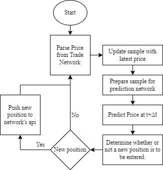
General overview flowchart for the cryptocurrency trading AI

A general overview of the trading algorithm.

Interface Layers

Input Layer

The input layer connects to an exchange and requests price data on a fixed cadence. Exchanges such as Binance expose HTTP and socket APIs; for this implementation, HTTP request–response against Binance endpoints was sufficient, using the publicly available python-binance utilities for both live requests and the collection of training data.

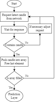
Input layer flowchart.

Once a minute, the latest one-minute candle is fetched and stored in a fixed-length buffer sized to the prediction model's window: new candles are pushed to the front and the oldest dropped, so the history cycles while staying the same length. The system does not begin predicting until the buffer fills. If a response is malformed or delayed past the sample rate, the layer retries and back-fills missed candles; alternatively it can request n candles at once to avoid the warm-up wait, at the cost of a larger, slower response.

Output Layer

The output layer places orders. It holds the current position in memory and compares it against incoming decisions: if the decision layer calls for a long while the system is already long, no new order is sent. Because the model does not forecast exact prices, only market orders are used, and positions are kept small and uniform so they fill quickly, minimize slippage, and avoid moving the market — which would undermine the prediction the trade was based on.

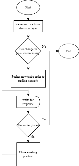
Output layer flowchart.

After pushing an order the layer waits for the exchange's response. On success it updates its internal state and hands control back to the input layer; on any other response it attempts to close the position and reset, so a failed-but-open position does not bleed money.

An unideal interface

Much of the design follows from the fact that trading through an API is imperfect. Three properties dominate. First, there is request–response latency — well over 100 ms between Canada and an exchange — so trades must be enacted quickly before conditions move; a minimum trade duration absorbs this. Second, the system does not know the exact fill price, which rules out limit orders (a limit order may fill slowly, partially, or not at all, and would require follow-up requests), so market orders are preferred. Third, market orders incur slippage: a market buy walks up the order book, filling against progressively worse prices, by an amount that depends on size and conditions. Limiting position size keeps fills fast, consistent, and low-impact.

Prediction Approach

The prediction layer takes a sequence of recent states and forecasts future ones. Before any network sees the data, the input is conditioned to suppress its random-walk character, and a representation is chosen that exposes structure across both time and scale. This section describes the rationale for those choices; the realized layers, loss, and training are detailed in the Wavelet GAN Trading Prototype.

Robust reweighting

Even with a tight zero-centred increment distribution, the price can jump sharply over short intervals, and a window containing such an event has skewed statistics that hurt prediction. Each observation is therefore reweighted with a Huber weighting derived from a scaled residual: the scale factor is the median absolute deviation rescaled by $1/0.6745$, and the residual is the absolute deviation from the sample median. The median is robust to outliers and unique to each window; because each window is expected to be near zero-mean, zero can stand in for the median.

$$ SF = \frac{\text{median}(\text{abs}(X_i - \text{median}(X)))}{0.6745} $$ $$ \text{Residual} = \frac{\text{abs}(X_i - \text{median}(X))}{SF} $$ $$ W_i = \left\{\begin{matrix} 1, & \frac{\left | X_i - \text{median}(X) \right |}{SF} \leq 1.547 \\ \frac{1.547}{\left | X_i \right |}, & \text{otherwise} \end{matrix}\right.$$

(Akram et al.)

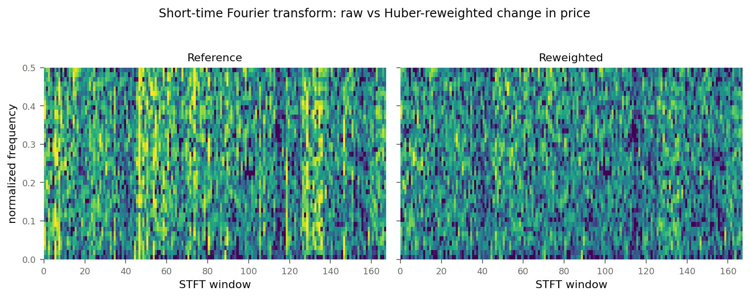
Huber weighting is preferred over harder estimators because reweighted samples group more tightly around zero with smaller variance without detrending the signal — it leaves in-range values untouched and only pulls in outliers, preserving the trend information a trader needs. Comparing the short-time Fourier transform of a sample before and after reweighting shows the high-energy bands that mark statistical anomalies disappearing, and the per-window spectra becoming more uniform.

Short-time Fourier transforms of a reference (left) and Huber-reweighted (right) seven-day sample of one-minute price changes; the reference shows bright anomaly bands that the reweighting washes out. — Short-time Fourier transforms of a reference (left) and reweighted (right) seven-day sample of one-minute price changes. Reweighting removes the anomaly bands and evens out the per-window spectra.

Why wavelets, and which one

For samples close together in time, similarity of frequency content extends to similarity of spectral density: the magnitude of the Fourier transform of one window approximates that of a nearby window. Treating spectral content as the prediction target gives the network more to work with than a raw sequence.

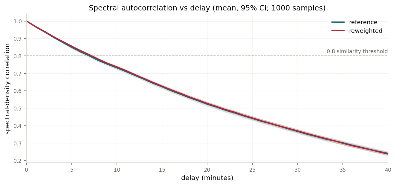
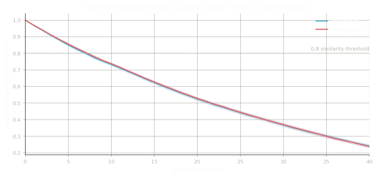
Correlation between a window's spectral density and that of a later window, against delay; reference and reweighted curves with 95% confidence bands, averaged over one thousand samples. — Autocorrelation of sample spectral density (reference and reweighted), averaged over one thousand samples with 95% confidence bands. Similarity stays above 0.8 for roughly a tenth of the 80-minute window.

Using an 0.8 autocorrelation threshold for "similar," nearby windows stay similar for roughly a tenth of the window size — enough to justify short-horizon prediction. A wavelet transform is preferred over the Fourier transform for the representation itself: it localizes in time through compact support, resolves several frequency bands at once, and makes low-pass filtering trivial (dropping the levels that carry high-frequency content). For a transform to be usable here, the original sample must be recoverable by its inverse to within a tiny error.

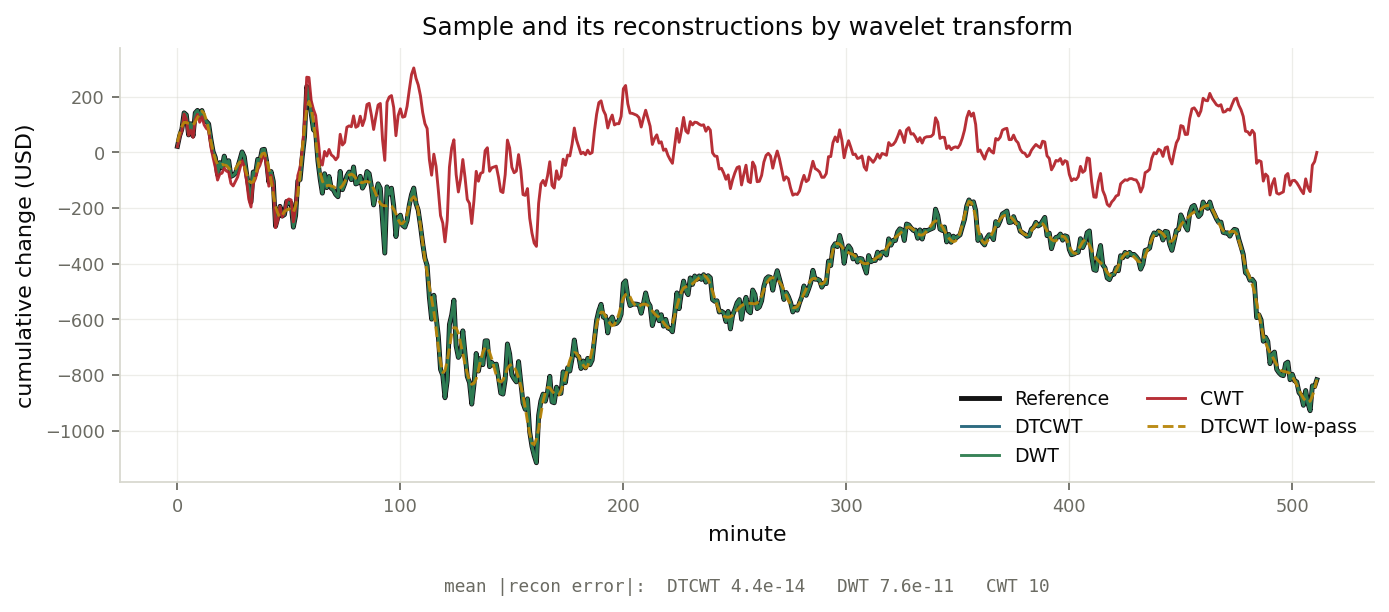
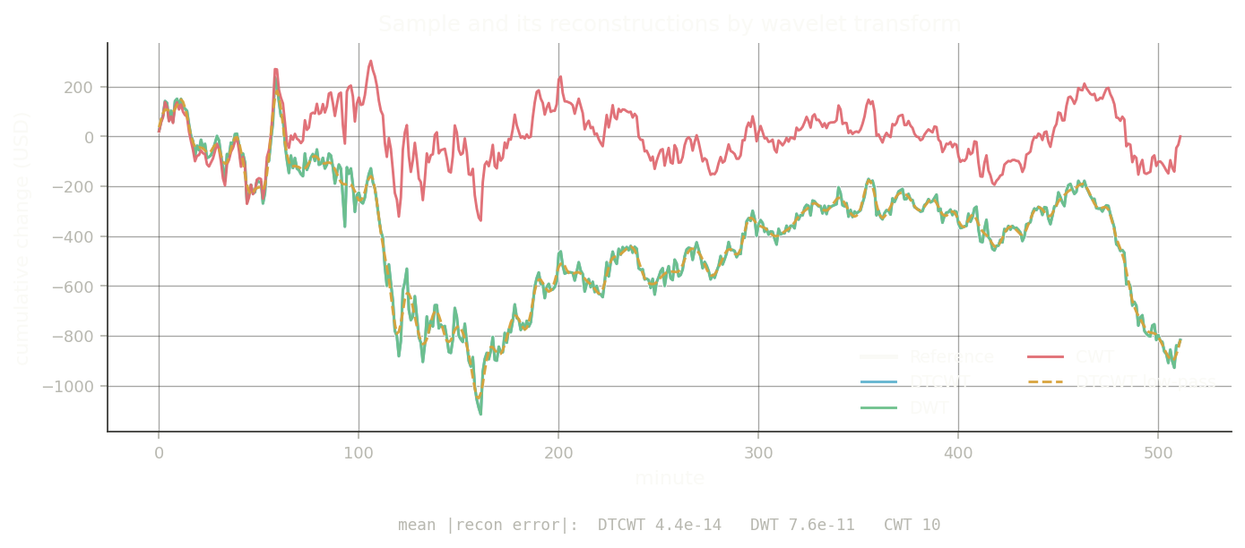
Cumulative sums of a sample and its reconstructions by the continuous, discrete, and dual-tree complex wavelet transforms; the DWT and dual-tree reconstructions overlap the reference while the CWT reconstruction diverges. — Cumulative sums of a sample and its reconstructions. The reference, DWT, and dual-tree complex reconstructions overlap almost exactly; the CWT reconstruction does not (mean reconstruction error: DTCWT 4.4e−14, DWT 7.6e−11, CWT ~10).

Three transforms were compared by mean reconstruction error $\zeta$ over one thousand eight-hour samples: the continuous wavelet transform (8.68), the discrete wavelet transform (3.122e−7), and the dual-tree complex wavelet transform (4.016e−14). The CWT is a superb analysis tool but detrends by subtracting a high-order polynomial whose accuracy decays outside the window and whose parameters it does not return, so reconstruction suffers. The dual-tree complex wavelet transform wins on two counts that matter for a sequence-to-sequence task: near-exact reconstruction, and approximate shift invariance, so that the decomposition at time $t$ is close to the one at $t+1$. It also produces redundant real and imaginary channels the network can exploit. The dual-tree transform is adopted throughout.

$$ \Psi_c(t) = \Psi_r(t) + j \cdot \Psi_i(t) $$

(Selesnick et al.)

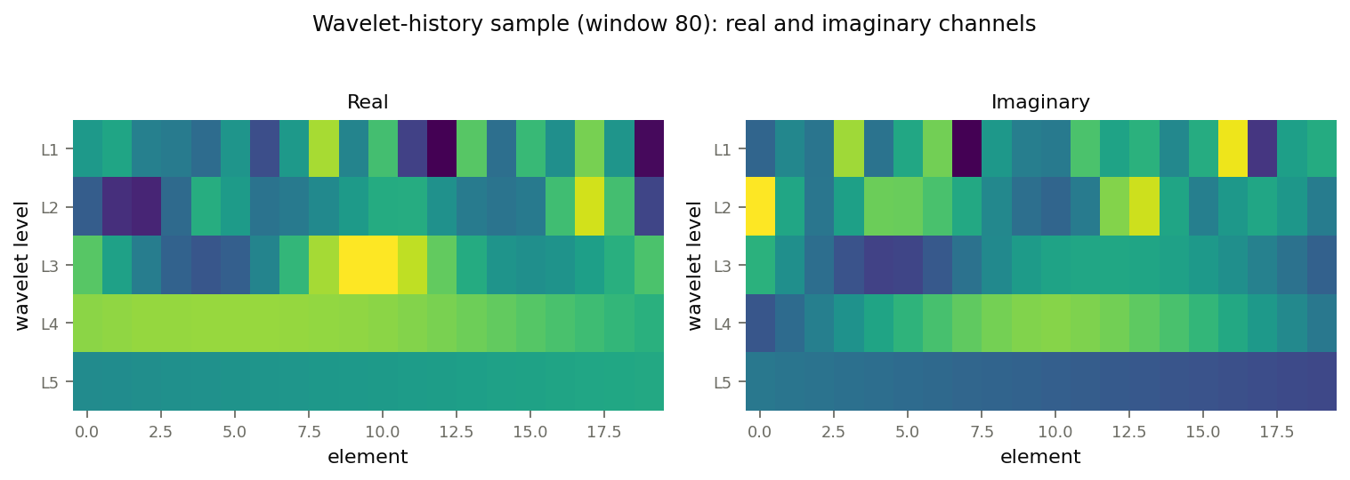
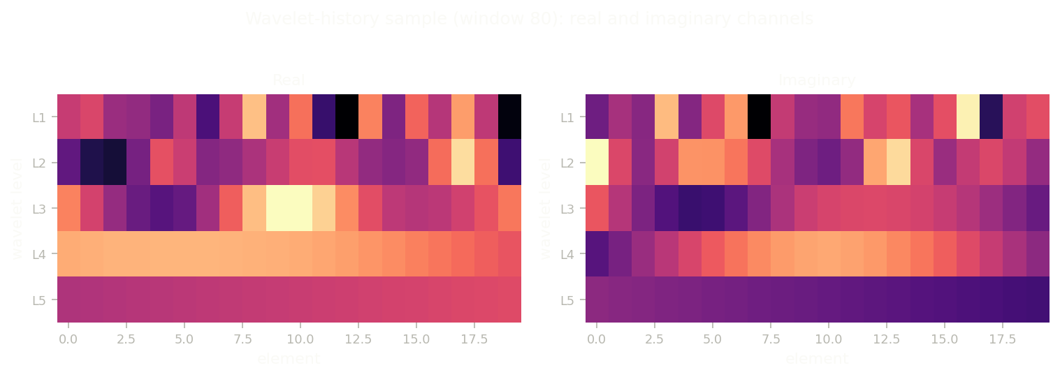
Before reaching the network, a window is reweighted, decomposed with the dual-tree transform, low-pass filtered, and rearranged so that decomposition levels sit side by side in a two-dimensional array, with real and imaginary parts stacked along a third dimension. Levels beyond the first are interpolated to a common length using Akima spline interpolation, which assumes little about the data and handles complex values well. Scaling coefficients change slowly between adjacent steps and are carried forward rather than predicted.

Real and imaginary channels of a dual-tree wavelet-history sample for an 80-minute window, arranged by decomposition level. — Real and imaginary channels of a dual-tree wavelet-history sample (window size 80), arranged by decomposition level — the structured input the network receives.

The Kalman analogy

No model is perfect, and the price at any instant may sit above or below an "ideal" value because of euphoria or panic. Treating the market price as an ideal price plus noise is a useful framing.

$$ \text{price} = \text{idealprice} + \text{noise} $$

A Kalman filter, given the statistics of that noise and the previous state, recovers a near-real-time estimate of the true state — exactly the property needed to keep consecutive predictions stable as fresh, noisy data arrives. A literal Kalman filter, however, struggles when the system's dynamics change quickly, as cryptocurrency markets do. Rather than bolt one on, the network is designed to develop its own equivalent: it receives its previous prediction alongside the latest observation, giving it the chance to correct itself, in the spirit of a state-update step.

$$ \hat{X}_{k+1}^{-} = f(\Theta,Z_k,\hat{X}_k^{-}) $$

An adversarial objective

There is a fundamental tension in trading on a forecast: acting on a prediction changes the system the prediction described. The moment a trade is executed, the market becomes one that includes the trader, and accuracy decays. Formally, the realized change in price combines a "natural" component with a component caused by the trade, scaled by an unknown influence $H$; only when the trade-induced change is zero does the realized change equal the natural one.

$$ \Delta P_t = \Delta P_{t,\mathcal{B}} + H \, \Delta P_{t,g} $$

Because that influence cannot be known in advance, chasing an exact prediction is self-defeating. The network instead learns to generate plausible futures consistent with the signal's stochastic structure, which is precisely what a conditional generative adversarial network is good at. The generator proposes a future window; a discriminator learns to tell generated futures from real ones; together they push the generator toward outputs statistically indistinguishable from genuine continuations.

$$ G^* = \text{argmin}_G \; \text{argmax}_D \; \mathcal{L}_{cGAN}(G,D) + \lambda \mathcal{L}_{L1}(G) $$

(Isola, 3)

This is the conceptual heart of the system. The concrete generator and discriminator — grouped convolutions over the wavelet-history tensor, the compound adversarial-plus-reconstruction loss, and the training schedule that refreshes samples across the dataset to fit in memory — are specified and evaluated in the Wavelet GAN Trading Prototype, and exercised end-to-end across 30-, 60-, and 128-minute horizons in the WaveGAN BTCUSDT Extrapolation Report.

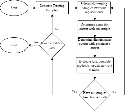
Training routine flowchart showing sample refresh across epochs

Training routine: new samples are generated each epoch and swapped into the training set so the network sees the whole dataset under a fixed memory budget.

Decision Layer

With a forecast in hand, the system still needs a rule for when to enter and exit. Because it can hold either a long or a short, it can in principle profit from both up- and down-trends; the difficulty is converting noisy forecasts into trades without churning. Three approaches were proposed, in increasing sophistication: combining several overlapping forecasts with the same robust M-estimator used for outlier removal; applying a profit-tuned low-pass filter to the recovered forecast and trading on its slope; and training a network to map price data directly to the long/short signal that would have maximized historical profit (constructed by recursively inserting trades at the most profitable local extrema, subject to a minimum spacing). On Bitcoin's data the tuned rule favoured a thirty-minute minimum spacing and a filter removing the top 15% of frequency content, giving an average trade duration near nineteen minutes.

This is the least developed part of the proposal, and deliberately so: the rest of the series narrows to the forecasting question and never returns to the trading decision. Early decision networks (bidirectional LSTM stacks) fit the training data but generalized poorly out of sample — the same difficulty the later forecasting studies set out to characterize.

Afterword

As demonstrated on Bitcoin, the combination of wavelets and generative adversarial networks can extrapolate a random signal with reasonable fidelity — owed to the GAN's ability to reproduce a signal's stochastic distribution and the wavelet transform's ability to expose structure across scale. Because such a forecast is a plausible scenario rather than an exact one, it suits a setting like trading, where the act of trading changes the future being predicted.

The decent simulator results should be read with care. A real market responds to orders; the historical simulator does not, so its market is unaffected by the system's actions. That gap is exactly why these results carry little weight for live deployment. Taken honestly, the contribution of this proposal is conceptual: it shows the idea is coherent and worth testing, and it defines the system whose forecasting pieces the rest of this series builds and measures — the WaveGAN experiment, the Wavelet GAN Trading Prototype, and the Wavelet Feature Forecasting Study.