Wavelet-Conditioned Generative Adversarial Networks for Extrapolating Stochastic Price Signals.
Case Study: Bitcoin Price-Change Forecasting for Algorithmic Trading Research.
Abstract
Financial markets are noisy, adaptive systems, and continuous-function models are often only local approximations. Structured models such as geometric Brownian motion or adaptive-belief systems are useful references, but their assumptions can weaken when trader behaviour, volatility, or liquidity regimes shift. This report frames volatile-asset prices as nonlinear stochastic dynamics and studies a wavelet-conditioned GAN prototype for extrapolating short windows of Bitcoin price-change data. The work should be read as a research prototype: it compares real and synthetic data, documents the architecture and loss construction, and reports early validation results rather than making a live-trading claim.
This is the architecture-and-evaluation deep dive of the series. The motivation and the empirical premise are established in the Trading AI Proposals, and the first end-to-end MATLAB build is the WaveGAN BTCUSDT Extrapolation Report; this page specifies the generator and discriminator in full and reports what held-out evaluation actually showed. Read it alongside the later Wavelet Feature Forecasting Study, which re-tests the same intuition under stricter controls and reaches a more sober conclusion.
1. Introduction
1.1 Market Modeling Background
Financial markets, especially highly volatile cryptocurrency markets, often show random-walk-like behaviour. Many price drivers are difficult to observe directly, and attempts to measure them can lag or miss regime changes. Even so, short-horizon price changes can sometimes be treated as samples from a stochastic process. Black-Scholes is a useful reference point: it models an asset price under geometric Brownian motion with constant drift and volatility (Zhang 2), leading to the differential equation below.
Here S denotes price, W is a Wiener process, and μ and σ denote drift and volatility. The assumption is convenient, but limited: market volatility is not constant in practice.
Hommes (2001) gives a richer reference by modelling financial markets as nonlinear adaptive-belief systems with heterogeneous trader types and competing strategies. That framing is useful here because it treats market structure as endogenous and time-varying rather than fixed.
Here F is a nonlinear mapping, Xt is a price vector, njt is the fraction or weight of investors of type h, λ is a parameter vector, and δt and ϵt are noise terms (Hommes 6).
1.2 Limits of Structured Market Models
These structured approaches still assume a market form. In adaptive-belief settings, a structure that describes one regime may fade in the next. Analytical abstractions can be useful, but any live model needs to adapt quickly enough for changing market conditions.
Where X is a vectorized sample of S and Θk is a set of parameters.
1.3 Learning-Based Problem Framing
Under the working assumption that a useful finite-dimensional state representation exists, an asset price can be treated as a system whose future distribution depends on current and past states. The mapping described by Φ and Θ may remain useful while training and future data come from similar regimes. Neural parametrization reduces, but does not eliminate, assumptions about market structure: the model is asked to learn latent relationships rather than having them specified analytically.
Rather than assuming a literal true price, this report treats lower-frequency movement as an idealized component and short-horizon deviations as noise driven by slippage, localized panic, euphoria, and order-flow effects.
These high-frequency fluctuations are difficult to exploit after request-response latency, fill time, and slippage. Market orders reduce waiting time but can increase slippage, so the forecasting target is aimed at broader movement rather than every tick.
2. Concept
2.1 Forecasting Objective
Given a stochastic system with unobserved inputs, the proposed network learns how a distribution of future windows relates to the distribution of present and past windows. The goal is a plausible short-horizon continuation, not an exact price path. This is important in trading because the act of trading can change the state being forecast. Conditional generative adversarial networks are useful candidates for this framing because they can learn stochastic structure in data (Isola 7).
(Eq. 7 adapted from Isola 3)
Here Dk is a windowed set of price samples between t and t-ws, with ws denoting window size; Θk is the corresponding parameter set; G is a generator that synthesizes candidate future data; and D is a discriminator trained to distinguish reference samples from generated samples.
2.2 Temporal Conditioning
For temporal continuity, the network also receives its previous prediction. In an adaptive-market setting, the model may need periodic retraining or online fine-tuning as conditions change, but this report does not establish an additional online-learning mechanism. The proposed model is therefore a nonlinear mapping from parameters Θ, a windowed observation set D, and the previous prediction Xt-1 to a new prediction Xt (6).
3. Exploratory Evidence
3.1 Distribution of Candle-Level Changes
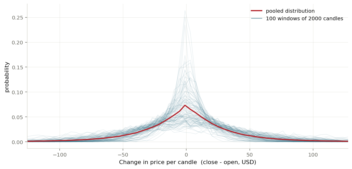
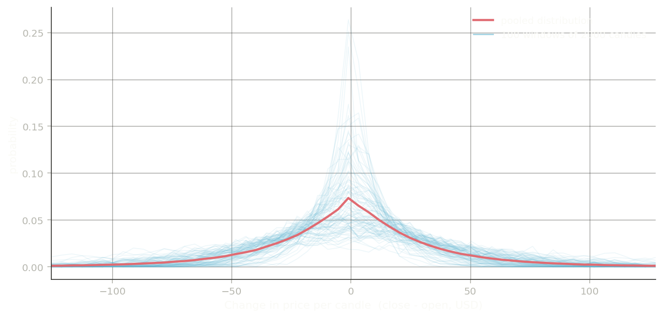
The design relies on candle-to-candle changes being describable, at least approximately, as a stochastic process. That premise — a near-invariant, zero-centred increment distribution beneath a random-walk price — is established at length in the Trading AI Proposals; the check here is a focused re-confirmation on the dataset used for this prototype. One hundred samples of two thousand candles were randomly selected from Bitcoin price data between 2021 and 2022, a period with relatively consistent trading volume. Probability distributions were created for each sample using histograms, and events with probability below 1e-3 were discarded.
Figure 1 shows the per-window distributions sitting almost on top of the pooled distribution. Across ten thousand random windows of two thousand candles (regenerated from the recovered dataset), the per-window mean stays near zero — mean −0.01, standard deviation 0.98 — while the per-window standard deviation averages roughly 44 USD with standard deviation 22. This does not prove stationarity, but it supports using roughly zero-centred, bounded-change windows in the prototype.
3.2 Spectral Variation Across Market Regimes
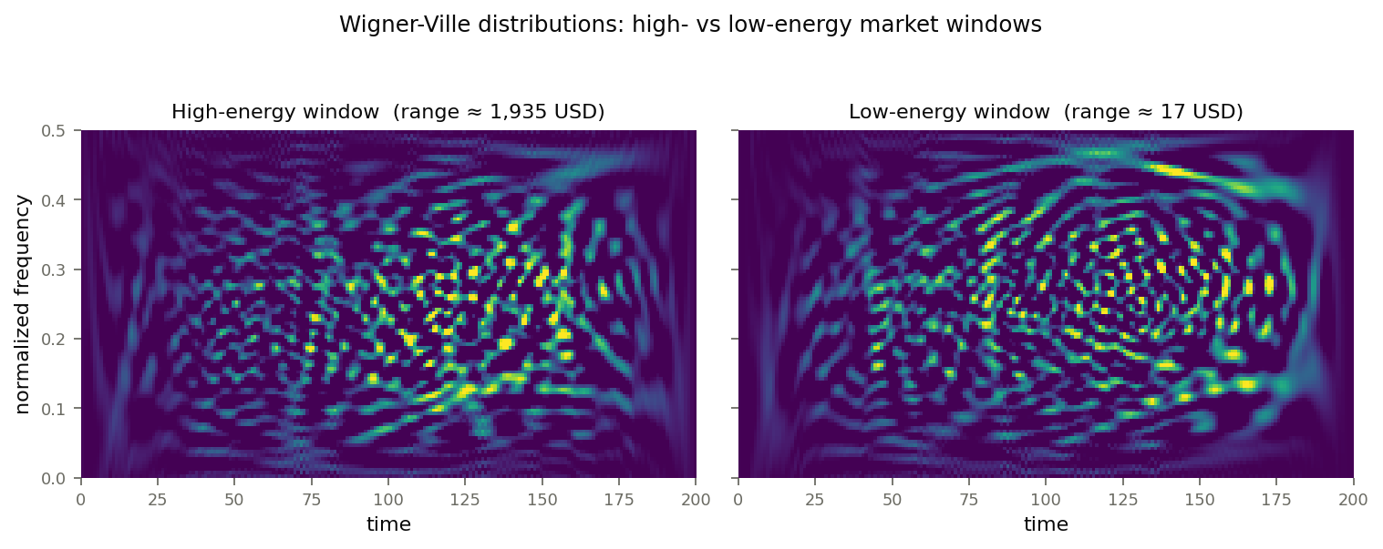
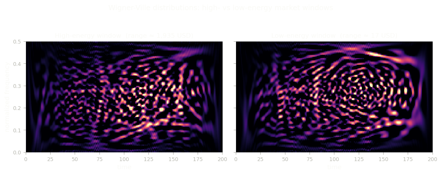
Market conditions still affect price changes, and those differences are visible in spectral content. To illustrate the effect, one high-energy and one low-energy sample were selected for comparison. Sample energy was calculated as the sum of the squared fast Fourier transform. From one hundred samples of one hundred candles, the samples with the highest and lowest energy readings were selected. The high-energy event corresponded to a high-volume trading scenario where price changed by more than one thousand USD within the sampled window. In the low-energy event, the total change across the sample was less than fifty USD.
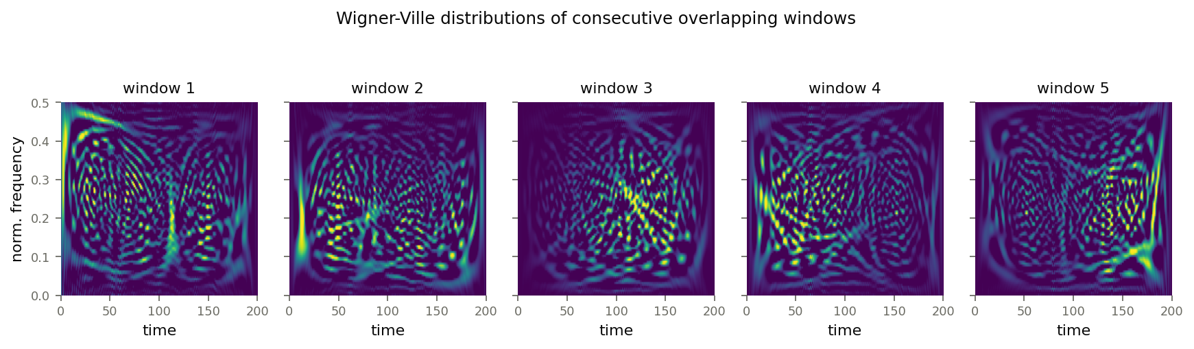
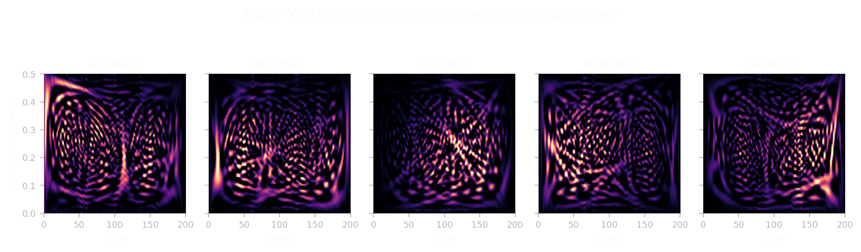
3.3 Continuity Across Consecutive Windows
4. Implementation
4.1 Wavelet Input Construction
The asset price is observed at a regular frequency and partitioned into samples with n observations. To expose lower-level structure and encode frequency information, samples are upscaled with the continuous wavelet transform (CWT).
4.2 Adversarial Objective and Loss Formulation
To expose system properties local to a sample time, the model retains a window of upscaled, wavelet-transformed signals. The encoder and prediction layers are intended to identify features shared across nearby sample windows while still responding to local market conditions. Generative adversarial networks are used because they can model stochastic variation, which is useful when price changes have random-walk-like behaviour but still show relatively stable distributional structure.
During training, the expected output plus a noise vector ζ is supplied in place of the network’s previous prediction. A noise set Dz and noise vector z are also supplied so the adversarial network is not forced into deterministic outputs (Isola 3). Equations 11-13 adapt the conditional-GAN objective from Isola et al. so it accepts sets of wavelet-transformed data (10) as inputs. They summarize the network-level learning target; several implemented sublayers have additional local targets.
Where a sublayer has a unique learning target, its loss function is described in the section for that layer. The compound loss that replaces equation 13 is denoted by equation 33; during training, equation 34 is used as the simpler implementation.
4.3 Generator Architecture
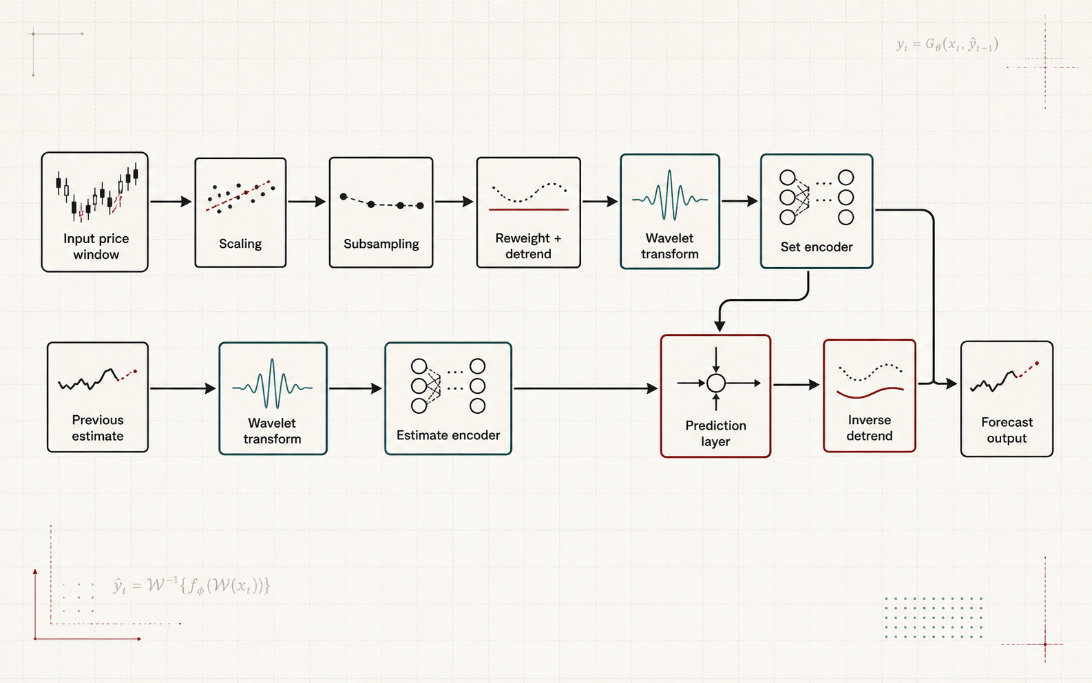
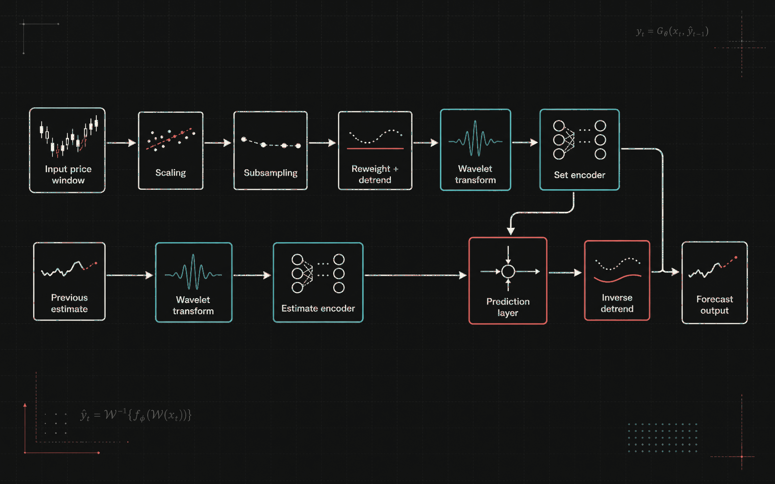
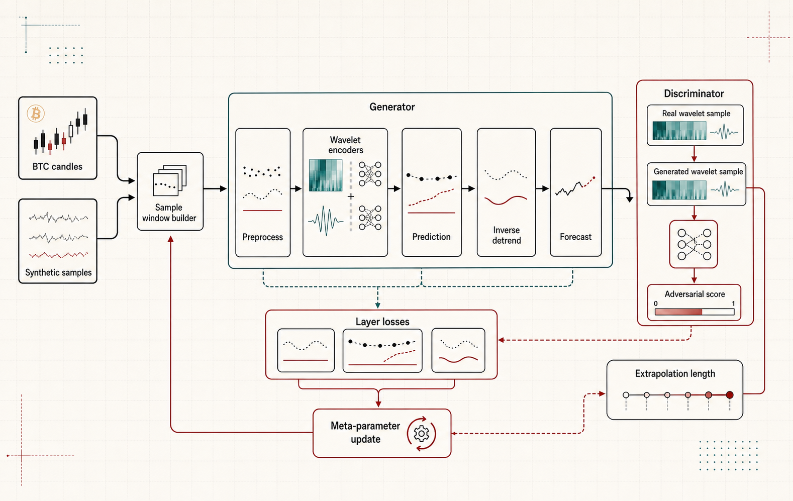
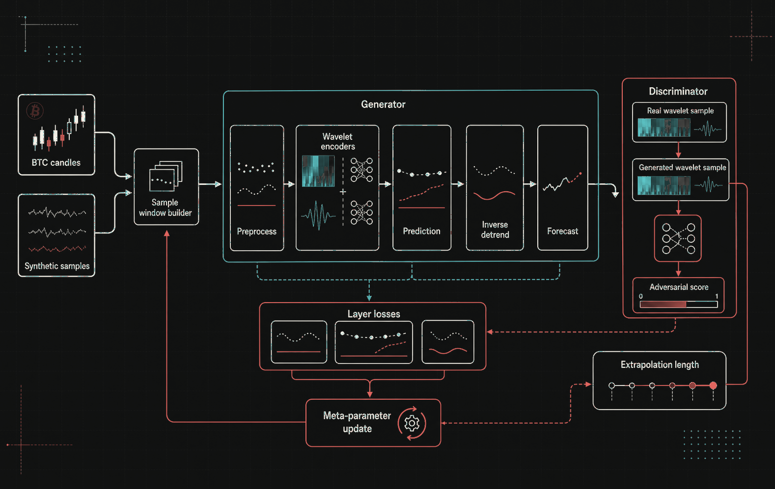
The implemented network is a generator-discriminator pair with several learning targets. The generator comprises eight layers: scaling, subsampling, reweighting and detrending, wavelet transform, set encoding, estimate encoding, prediction, and inverse detrending. It accepts one-dimensional samples of price-change data and outputs one-dimensional extrapolated continuations of the same signal. For temporal continuity, the generator’s previous estimate is also provided. Backpropagation is performed across the full generator, but selected layers also compute local losses before those losses are combined for gradient updates, which modifies the basic losses in equations 11 and 13.
The discriminator is a condenser-style network trained with PatchGAN-style loss. Because it accepts one-dimensional price signals, its inputs are transformed by the continuous wavelet transform before convolution. This encourages generated samples to resemble reference samples in spectral content.
4.4 Scaling Layer
This layer scales a large candle window so values fall roughly between -1 and 1. The number of candles it accepts depends on subsample window size, number of subsamples, and overlap between subsamples, as calculated in equation 14.
Here X is a candle-data vector containing nCandles. At the time of writing, each sample is divided by a scale factor. The scale factor is determined by fitting a normal approximation to X, then taking SF as the approximate 0.95 point of that fitted distribution.
4.5 Subsampling Layer
The subsampling layer rearranges the scaling layer’s output into a two-dimensional array of dimensions [WindowSize, nSubsamples]. Each sample overlaps the next according to the Overlap parameter. This converts a linear sample into a dataset sample and prepares the data for wavelet upscaling.
4.6 Reweight-Detrend Layer
Before data is upscaled with the continuous wavelet transform, preprocessing is used to preserve useful trend information and reduce the effect of outliers. The continuous wavelet transform convolves a signal with a sliding wavelet at changing dilations; each dilation corresponds to a wavelength. To focus on higher-frequency oscillations, the CWT implementation applies a detrending operation before convolution. Because it does not return the removed trend, the network needs a separate path for carrying that information forward.
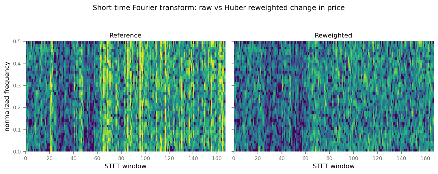
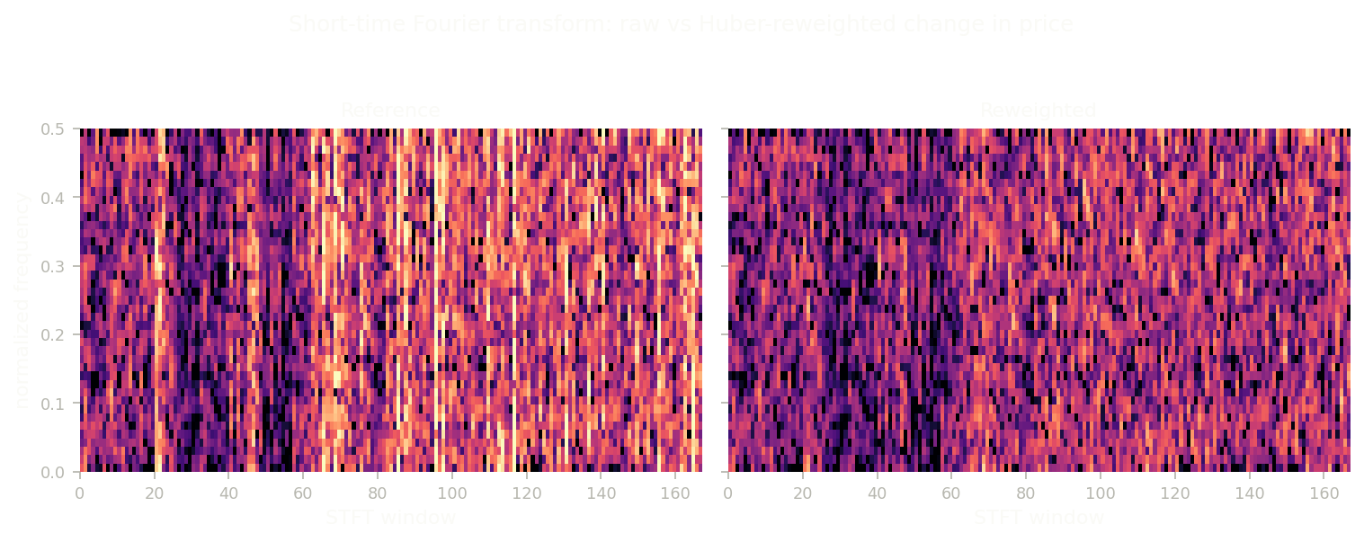
The dataset’s random-walk-like behaviour can skew sample statistics and reduce prediction quality. Figure 5 compares the short-time Fourier transforms (STFT) of raw (left) and reweighted (right) price data. In the raw data’s STFT, high-energy bands indicate outlying observations. Samples containing those points often look unlike regular samples, sometimes appearing almost flat with one or two peaks. Reweighting is therefore used to reduce the influence of those outliers.
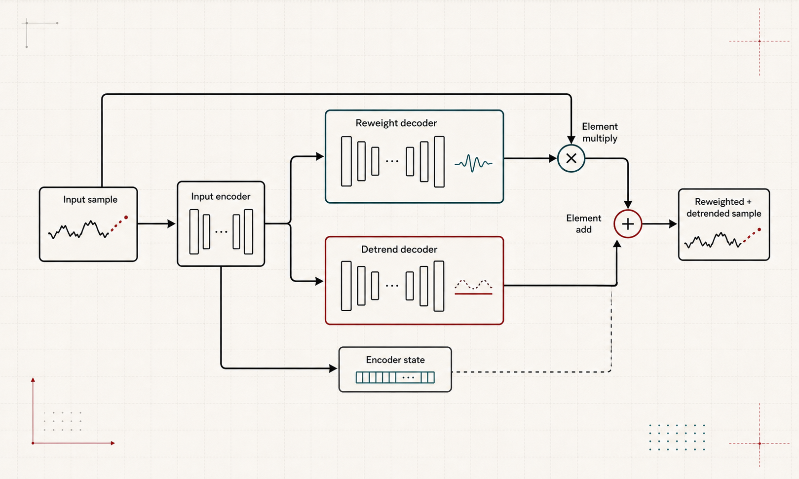
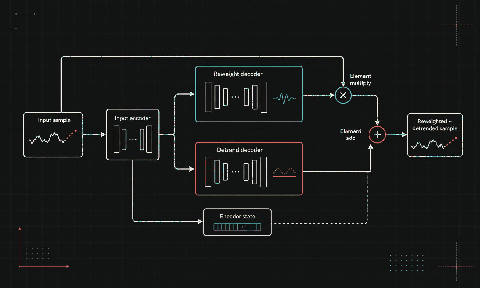
The reweight-detrend layer identifies outlying datapoints, applies a learned detrend, and returns information about those operations for later layers. Subsampled data first passes through an encoder, whose output is used to generate reweighting and detrending information in parallel. As illustrated in figure 6, the encoder uses repeating blocks of two one-dimensional convolutions with tanh activations followed by batch normalization. Its output is stored for the inverse-detrend layer. The detrend-decoder and reweight-decoder use matching stacks of transposed one-dimensional convolutions, tanh activations, and batch normalization. The reweight decoder output is multiplied element-wise with the original layer input, then added element-wise to the detrend decoder output.
The reweight-detrend layer has its own learning target. It minimizes Huber loss between the layer output and an empirical reference output, generated by reweighting the sample with Huber’s weight function and then applying the continuous and inverse continuous wavelet transforms in series (see equation 27).
To generate reference outputs for loss calculation, a scaled sample is reweighted with Huber’s weight function using a scaled residual. The scale factor is the median absolute deviation divided by 0.6745 (eq. 21), the residual is the absolute difference between an element and the sample median divided by that scale (eq. 22), and the residual determines the Huber weight (eq. 23). Akram et al. report this style of robust weighting as effective for identifying outlying datapoints.
(Equations 21-23, Akram et al. Equation 24, Beale et al.)
The Huber loss function computes loss according to equation 24 and defaults to δ = 1 (Beale et al. 1-759). Changing δ is beyond the scope of this investigation, so the default value is used throughout. The loss also sums across batches, which makes it compatible with the compound objective used for the generator.
4.7 Wavelet Layer
This layer upscales reweighted and detrended data by convolving it with a wavelet at different dilations, exposing time-frequency information about the signals. It converts batches of two-dimensional signal arrays into batches of three-dimensional frequency representations. The continuous wavelet transform is selected for its detailed time-frequency representation, and a Morse wavelet is used for convolution. The exact wavelet specifications are determined by the algorithm and depend on sample window size.
4.8 Set-Encoding Layer
The set-encoding layer uses grouped two-dimensional convolutions to extract features from consecutive samples’ spectral content. It splits the wavelet-layer output into real and complex components and concatenates them along the fourth dimension so model gradients remain real-valued. The layer then applies repeating blocks of two grouped two-dimensional convolutions with tanh activations and batch normalization. For compatibility with lower-dimensional layers, the grouped convolutions produce one singleton dimension, which is removed by squeezing the data.
4.9 Estimate-Encoding Layer
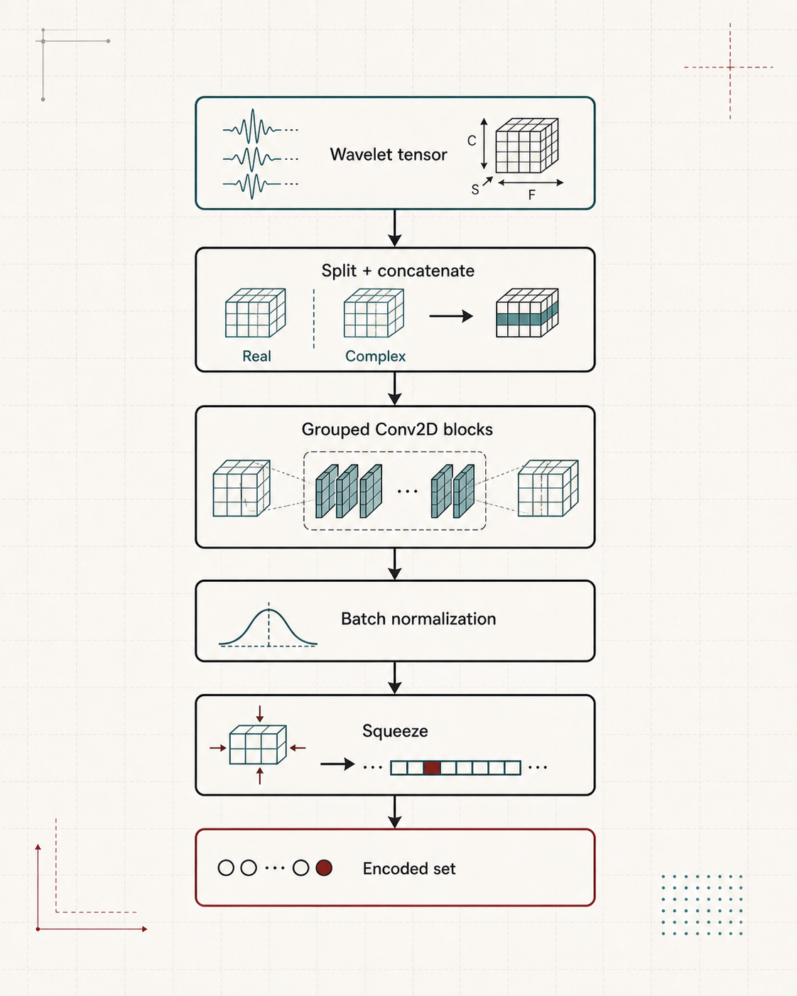
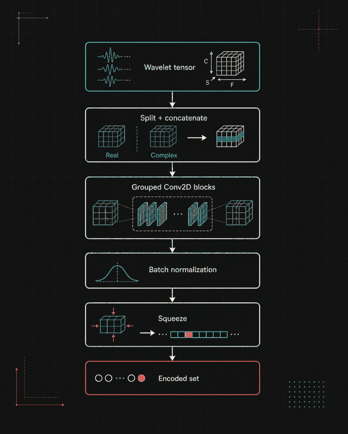
For continuity between consecutive predictions, the network also receives its previous prediction. The previous estimate is stored within the network object during use; during training, the last scaled and detrended input sample plus a noise vector is used instead. This layer calls the wavelet function to upscale the previous prediction for encoding. Apart from that wavelet step, the estimate encoder follows the set encoder’s architecture while handling fewer dimensions. See appendix A for a diagram.
4.10 Prediction Layer
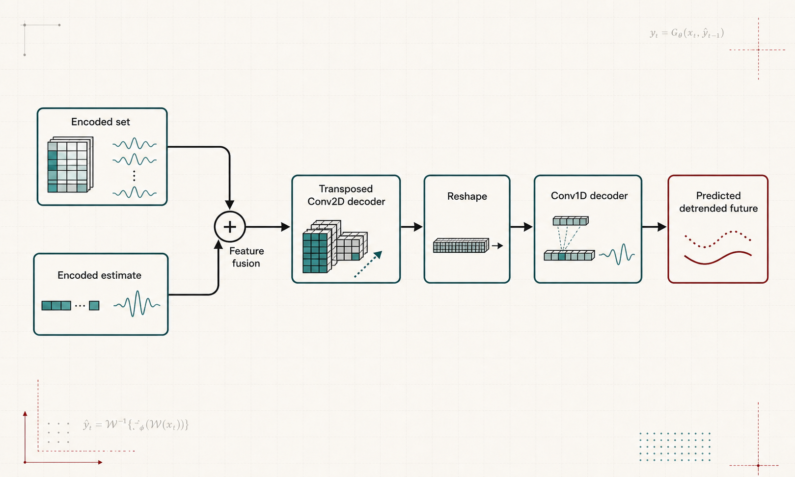
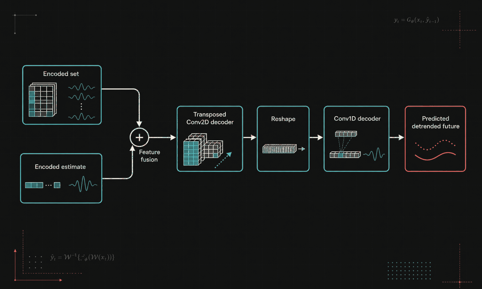
With the set and estimate encoders’ outputs as input, this layer predicts scaled and detrended future states. In effect, it maps the encoder outputs to a reweighted-detrended extrapolation (27). The layer has two decoders with similar convolution and batch-normalization blocks operating at different dimensionalities.
This layer also has its own learning target: matching the reweighted-detrended extrapolation. Huber loss is calculated according to equation 24, and reference outputs are generated with the same method used for the reweight-detrend layer. The output is scaled by the scaling layer before reweighting and detrending.
Here Xset and Xestimate are the set and estimate encoding layer outputs, ICWT and CWT are the inverse and continuous wavelet transforms, YRDT is the reweighted and detrended reference output from equation 27, and WHuber are Huber weights calculated with equations 21 through 23.
4.11 Inverse-Detrend Layer
The final generator layer, the inverse-detrend layer, uses information from the reweight-detrend layer to generate a trend vector, which is added to the prediction layer output.
This layer uses repeating blocks of transposed one-dimensional convolutions, with hyperbolic tangent activations, and batch normalization layers to generate the trending vector. The vector is then added to the detrended prediction to recover the trended signal.
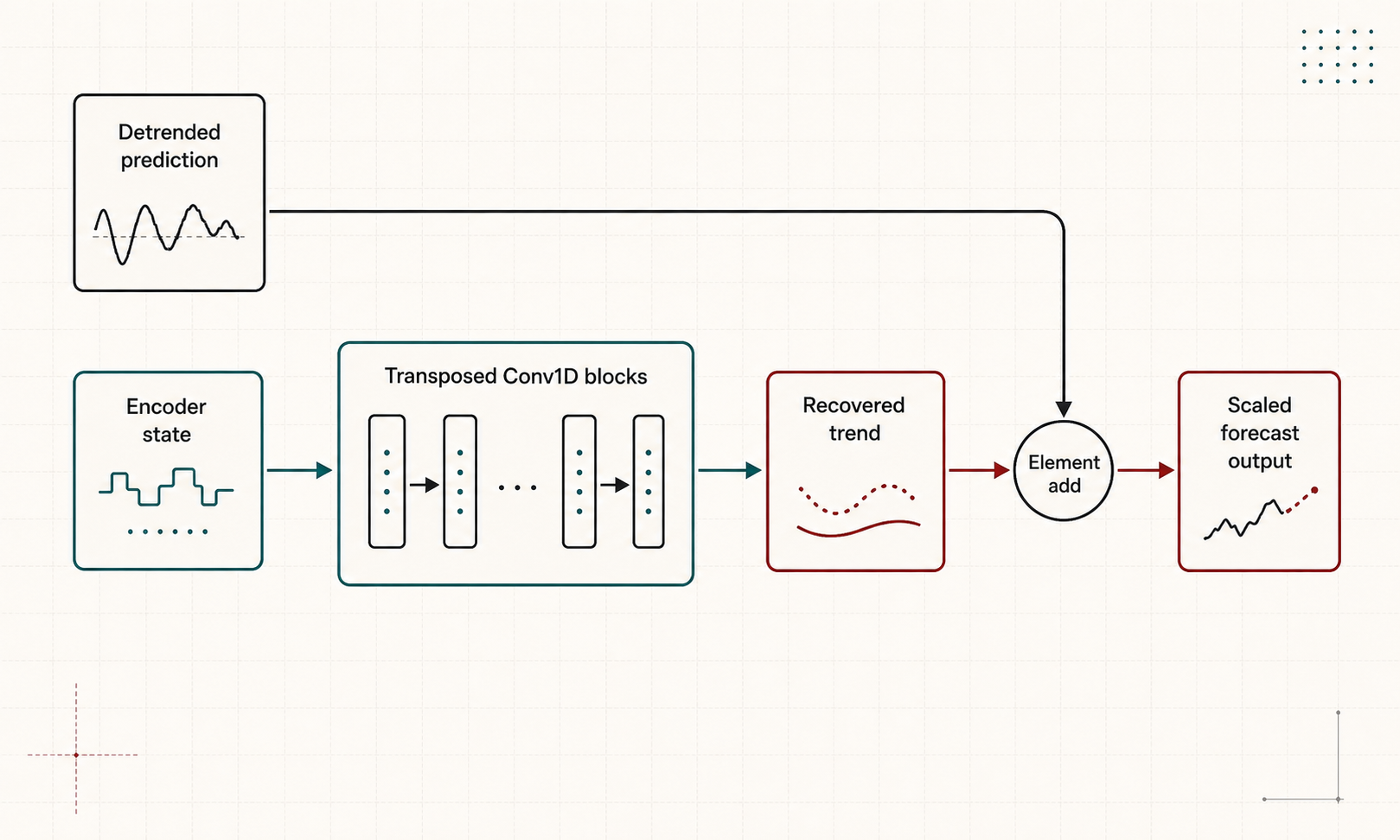
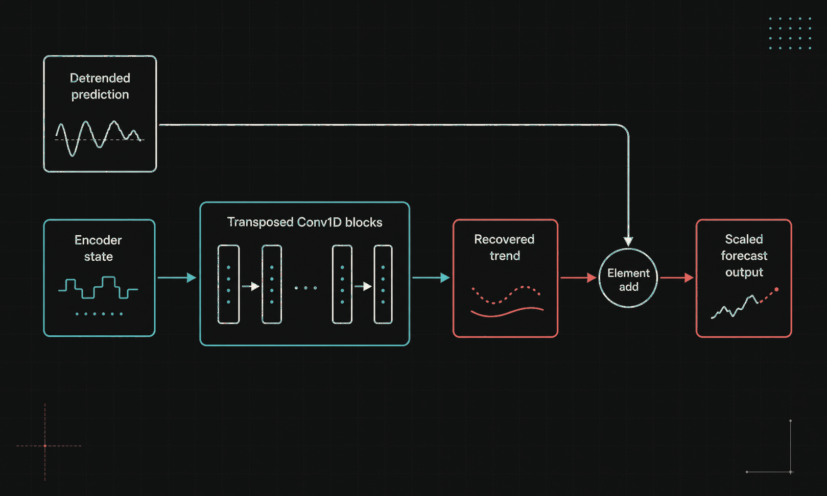
This layer also has a local learning target: minimizing error between its output and the scaled reference output. Like other locally supervised layers, its loss is smooth L1 (Huber) loss. The reference output is the windowed sample shifted forward by a fixed extrapolation length and scaled using the scale factor in equation 15.
4.12 Compound Loss Function
Because gradients are computed for the full network simultaneously, each local loss is combined into a generator loss that replaces equation 13. For ease of implementation, equation 34 is used instead of the more explicit equation 33.
4.13 Discriminator Architecture
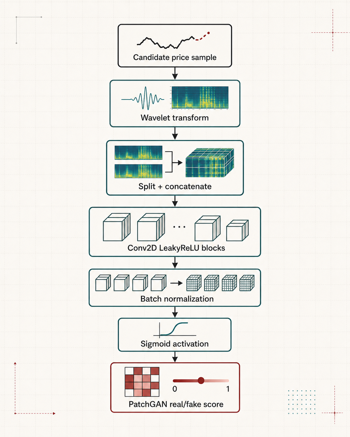
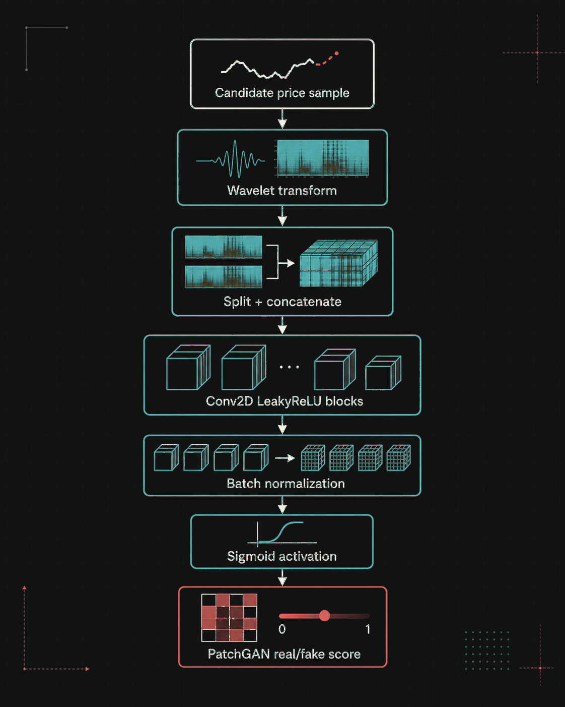
The discriminator encourages generated samples to match the spectral content of reference samples. It applies the continuous wavelet transform, then repeating blocks of two two-dimensional convolutions with leaky ReLU activations and batch normalization. A sigmoid activation maps the output between zero and one. Loss for this layer follows the adversarial term in equation 12.
4.14 Considerations for Training and Evaluation
During training, gradients are computed for each sublayer with respect to the adversarial loss described by equation 12, while equation 34 supplies the generator-side local loss in place of equation 13. In this gradient operation, the set and estimate encoders are treated as one sublayer.
Gradients are computed with Adam. Each sublayer, including the discriminator, has its own learning parameters, average gradient, and average squared gradient. Learning rates can differ between the generator and discriminator, though they were kept equal in this evaluation.
The model was evaluated at varying extrapolation lengths while holding window size, subsample overlap, and number of subsamples fixed. Those parameters determine how much local system information is available to the network.
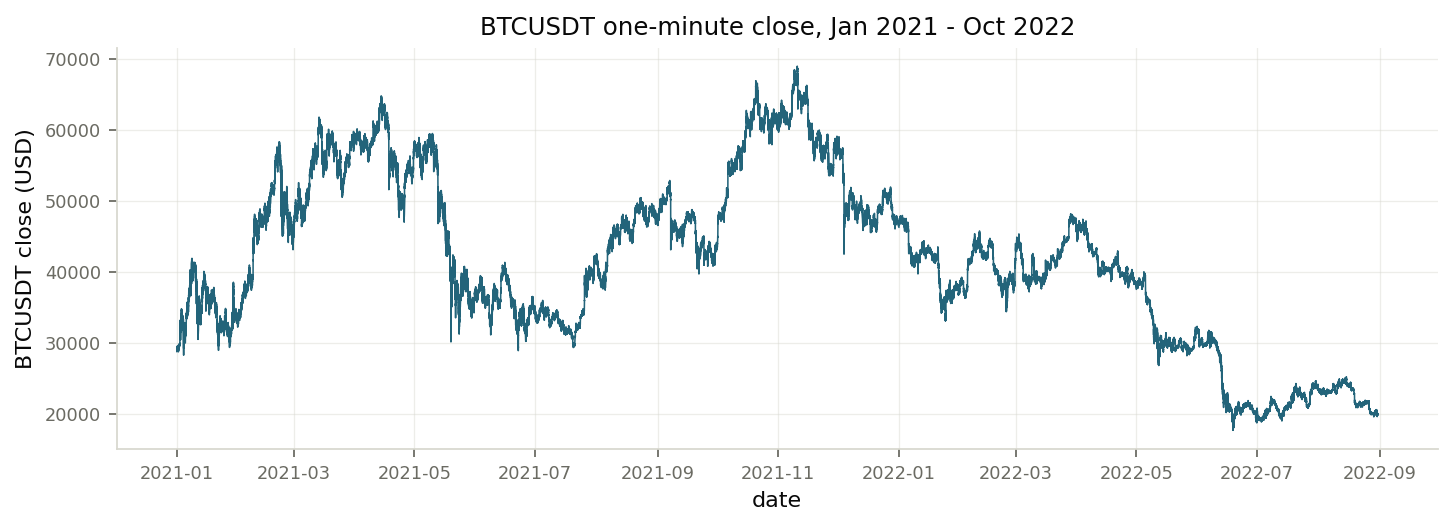
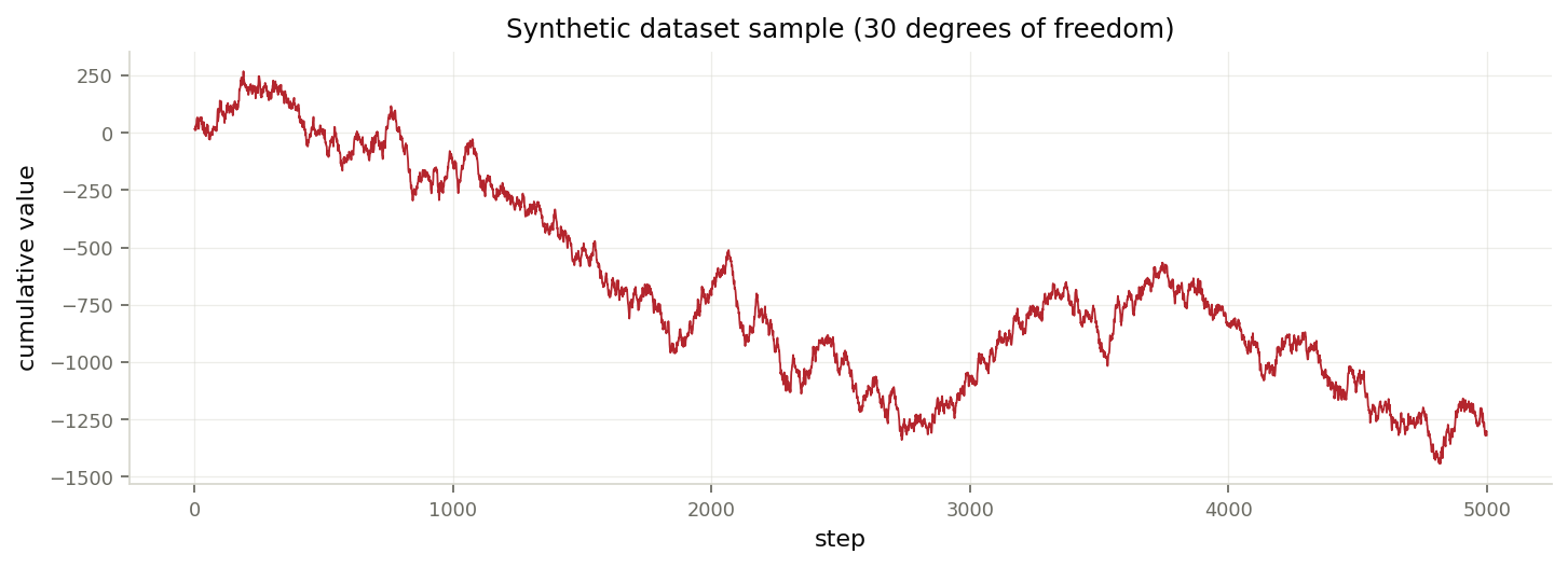
Evaluations used both real and generated datasets. The real dataset is Bitcoin price data from January 1, 2021, through October 1, 2022, sampled at one-minute intervals from Binance archives. Alternative datasets, each containing approximately one million samples, were generated according to equations 35-37 using 30 degrees of freedom.
When evaluating the model against configuration parameters such as window size and extrapolation length, datasets were randomly subsampled five thousand times. To evaluate performance on a larger real dataset, a loop generated new samples from the dataset at every epoch, giving the network broader exposure to the available market scenarios. Details of this loop are available in appendix A.
5. Evaluation
5.1 Extrapolation-Length Study
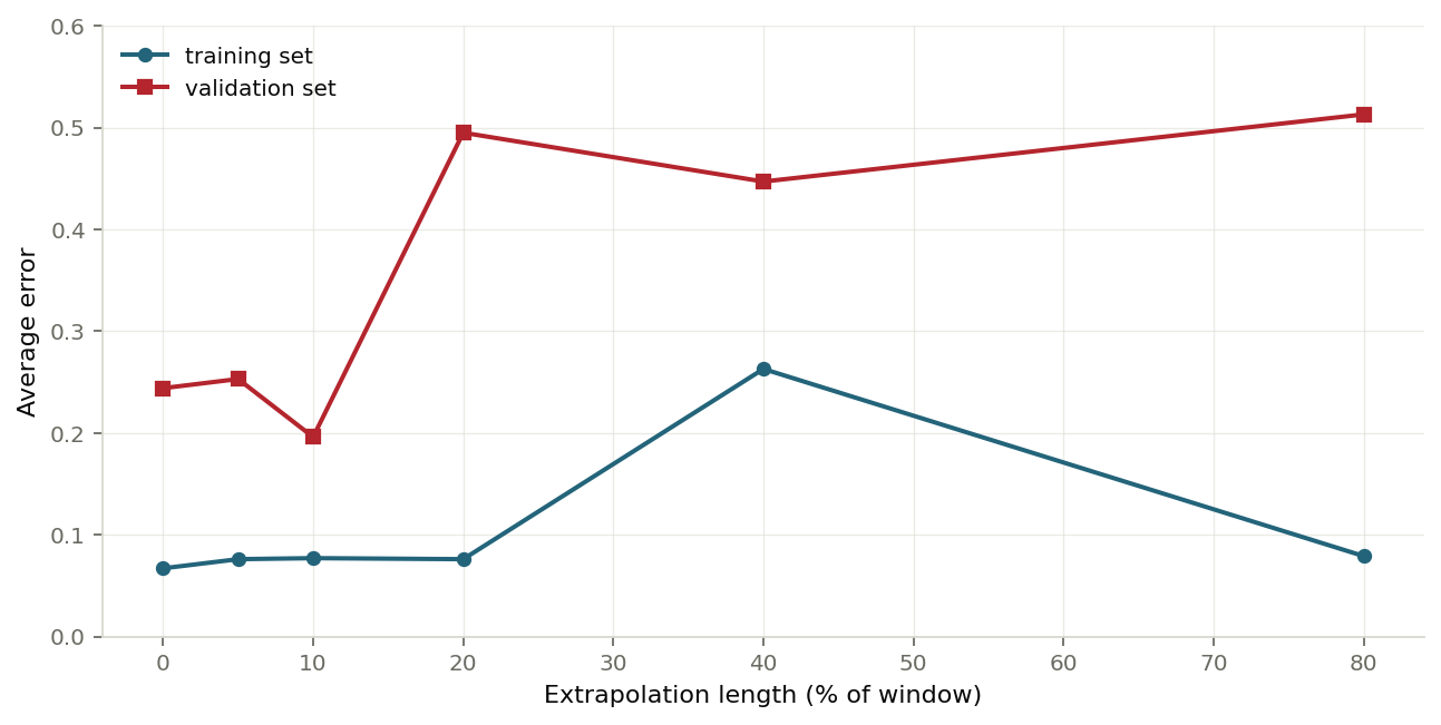
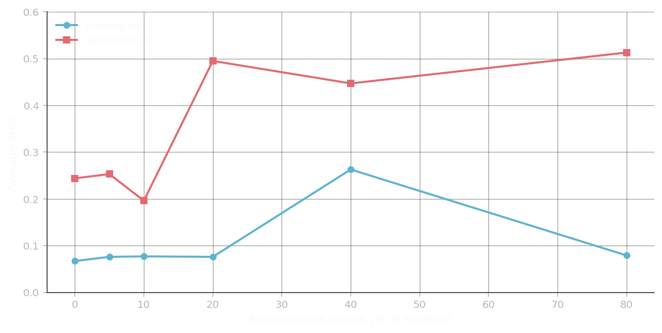
Hardware limitations restricted the configuration sweep, so the tested parameters are limited to the architecture in figure 11. Window size and overlap were set to 80 and 30 minutes respectively, while the number of subsamples was 30. Figure 12 reports results across several extrapolation lengths. The pattern is consistent with the earlier observation that the spectral content of a sample at time t + k becomes less similar to the sample at time t once k approaches roughly ten percent of the window size (Luna, 2022). An 80% extrapolation length was also tested with a much larger discriminator; in that run, the discriminator had approximately 1.5x more learnable parameters than the generator. After 297 epochs with five thousand training samples, average error was 0.079 on training data and 0.513 on validation data. Because the training and validation sets were sampled separately from the real dataset, the gap should be read as evidence of limited generalization. The larger-discriminator result suggests the discriminator may deserve more architectural attention, but it is not enough to establish an optimal design. For figure 12, training stopped when average error fell below 0.08 or after 300 epochs.
5.2 Synthetic-to-Real Transfer
When trained on data generated according to equations 35-37, the model produced broadly similar error profiles on real data as models trained directly on real samples. This supports the synthetic data as a rough stress-test input, but it does not validate the generator assumptions as a complete market model.
5.3 Held-Out Validation
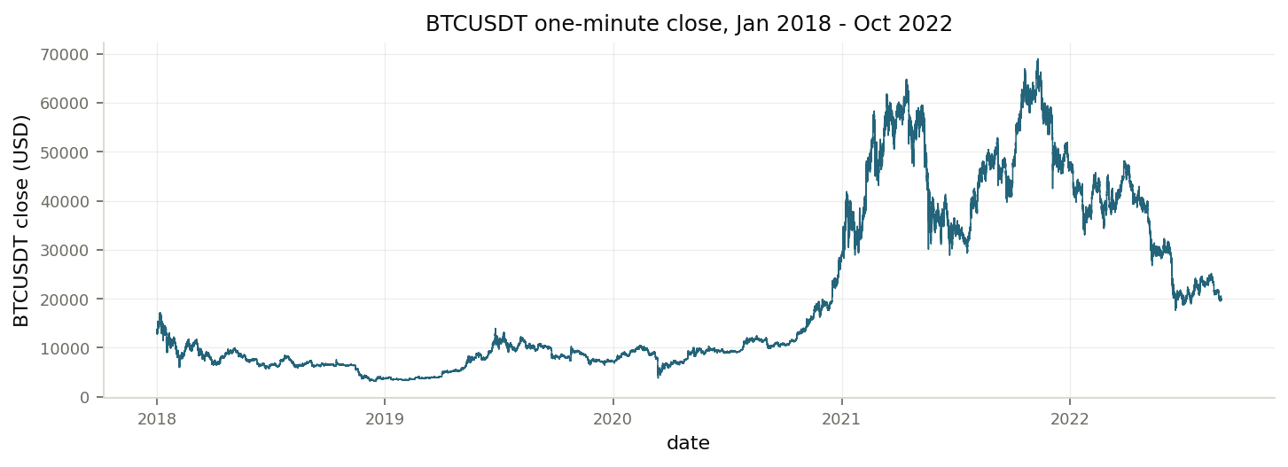
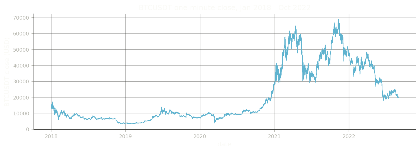
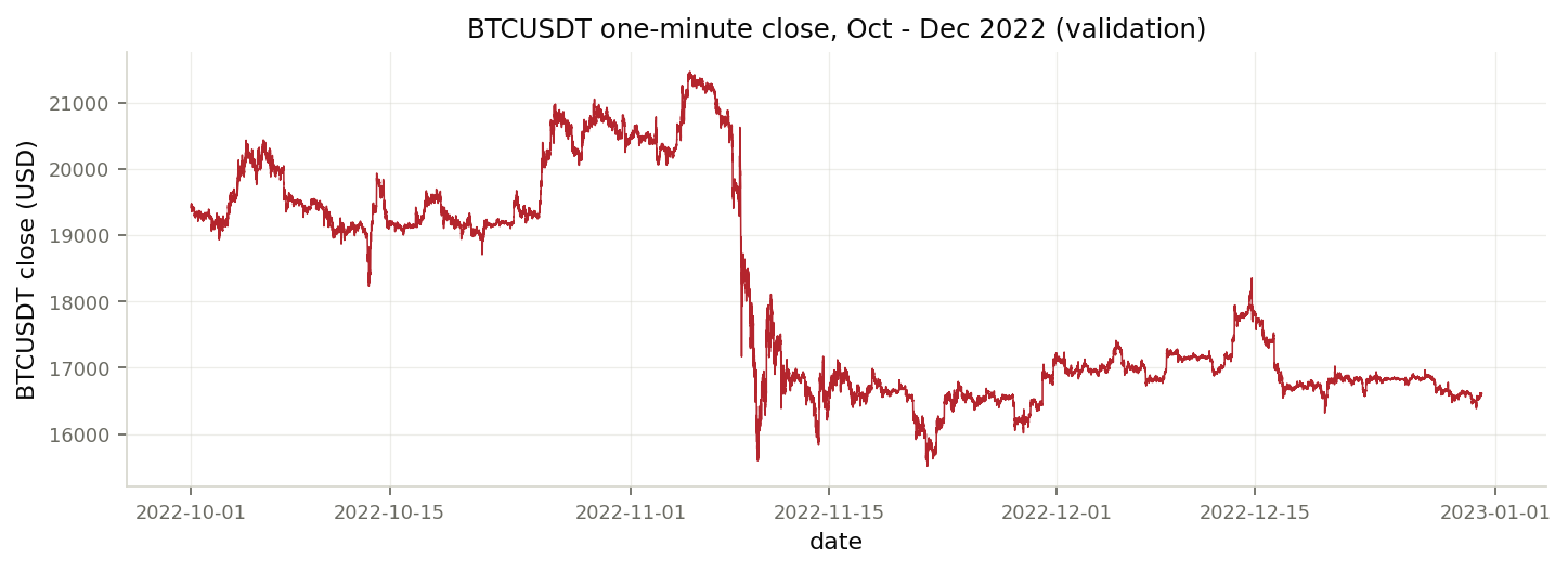
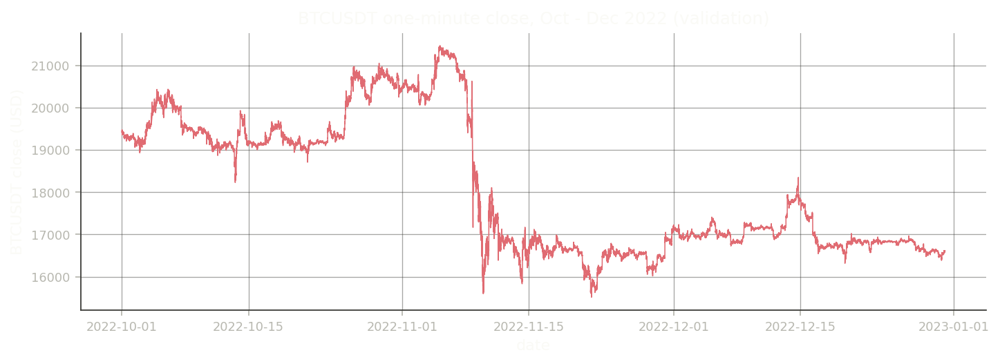
As a held-out check, the model was trained to extrapolate price data 20% of the sample window forward using one-minute candle data from January 1, 2018, through October 1, 2022. An earlier loop that drew five thousand random samples after each epoch caused extrapolated values to collapse toward zero with the figure 12 configuration. The validation run therefore used a fixed dataset of ten thousand randomly selected samples at 20% relative extrapolation length. After 410 epochs, average training error was 0.1355. Average errors on non-training samples drawn from the training-period pool and from the validation-period pool were 0.442 and 0.445 respectively. The validation period, unavailable during training, was one-minute candle data from October 1, 2022, through December 31, 2022.
Inspecting individual reference and predicted sequences — both the per-step series and their cumulative sums, split at the boundary between the observed window and the extrapolated region — shows the same story qualitatively. Over the known window the predicted path stays close to the reference; past the boundary the two diverge. On training-period examples the predicted cumulative path tracks the reference for longer before drifting, whereas on the held-out validation period the divergence sets in sooner and the cumulative paths separate more widely. That visible gap is the qualitative counterpart of the roughly 0.44-versus-0.1355 error difference between held-out and training samples.
6. Discussion and Outlook
Two things are established here. First, the wavelet-conditioned generator–discriminator is implementable as specified: the layer-local losses train, the compound objective is stable, and the network produces plausible transformed-domain extrapolations on data drawn from its training period. Second, and less comfortably, it does not yet generalize. The held-out run reached 0.1355 average training error but roughly 0.44 on non-training samples from both the training-period and the unseen validation-period pools, and the high-extrapolation run showed the same pattern (0.079 train versus 0.513 validation). The near-identical error on in-period-but-unseen and out-of-period samples suggests the limitation is generalization in general, not a clean train/test distribution shift.
It is worth being precise about what the error figures do and do not mean. They are computed on scaled, reweighted-detrended wavelet-domain targets, so a given value is a statement about transformed-domain reconstruction, not about time-domain price accuracy and certainly not about profitability. The architecture is best read as a careful feasibility study: it shows the representation and the multi-target training scheme work, and it surfaces the discriminator and the generalization gap as the parts that most need attention.
That diagnosis is what motivates the next part of the series. The Wavelet Feature Forecasting Study sets the GAN aside and rebuilds the question as a controlled forecasting benchmark — matched baselines, ridge regression, and residual temporal convolutional networks under fixed chronological splits and return-domain metrics. Under those stricter controls the simple baselines win, which reframes the contribution of this prototype: it demonstrated that the wavelet-conditioned design can be built and trained, while the later study showed that, on a fair benchmark, the added machinery did not yet beat the simplest reasonable comparators.
Appendix A: Additional Network Information
Estimate Encoding Layer Architecture Overview and Training Loop
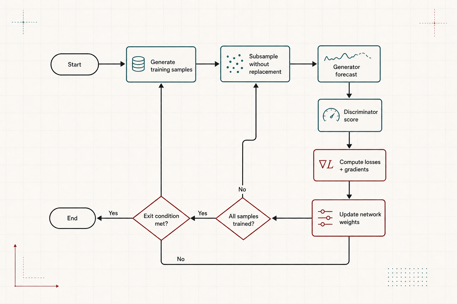
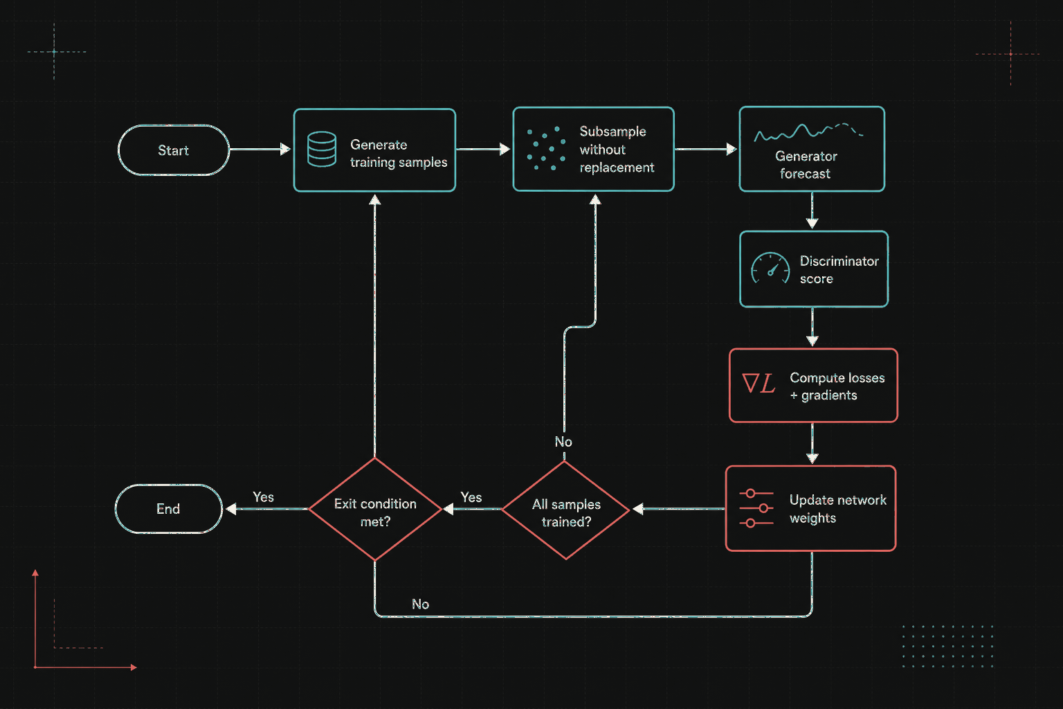
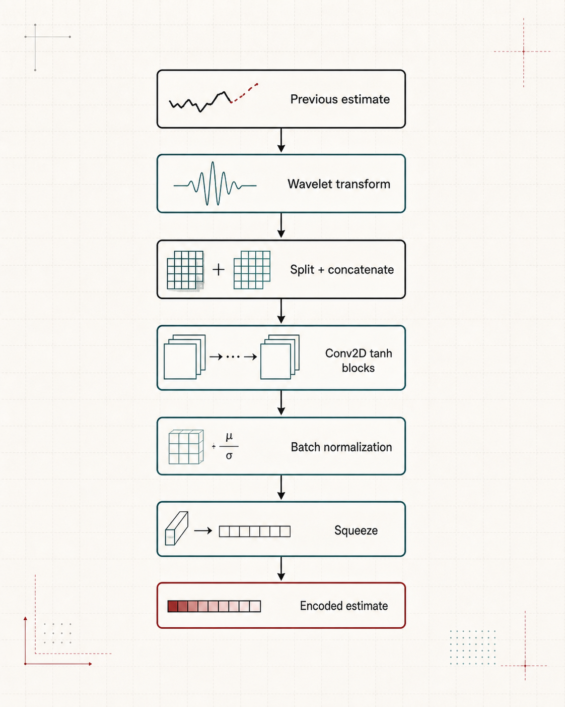
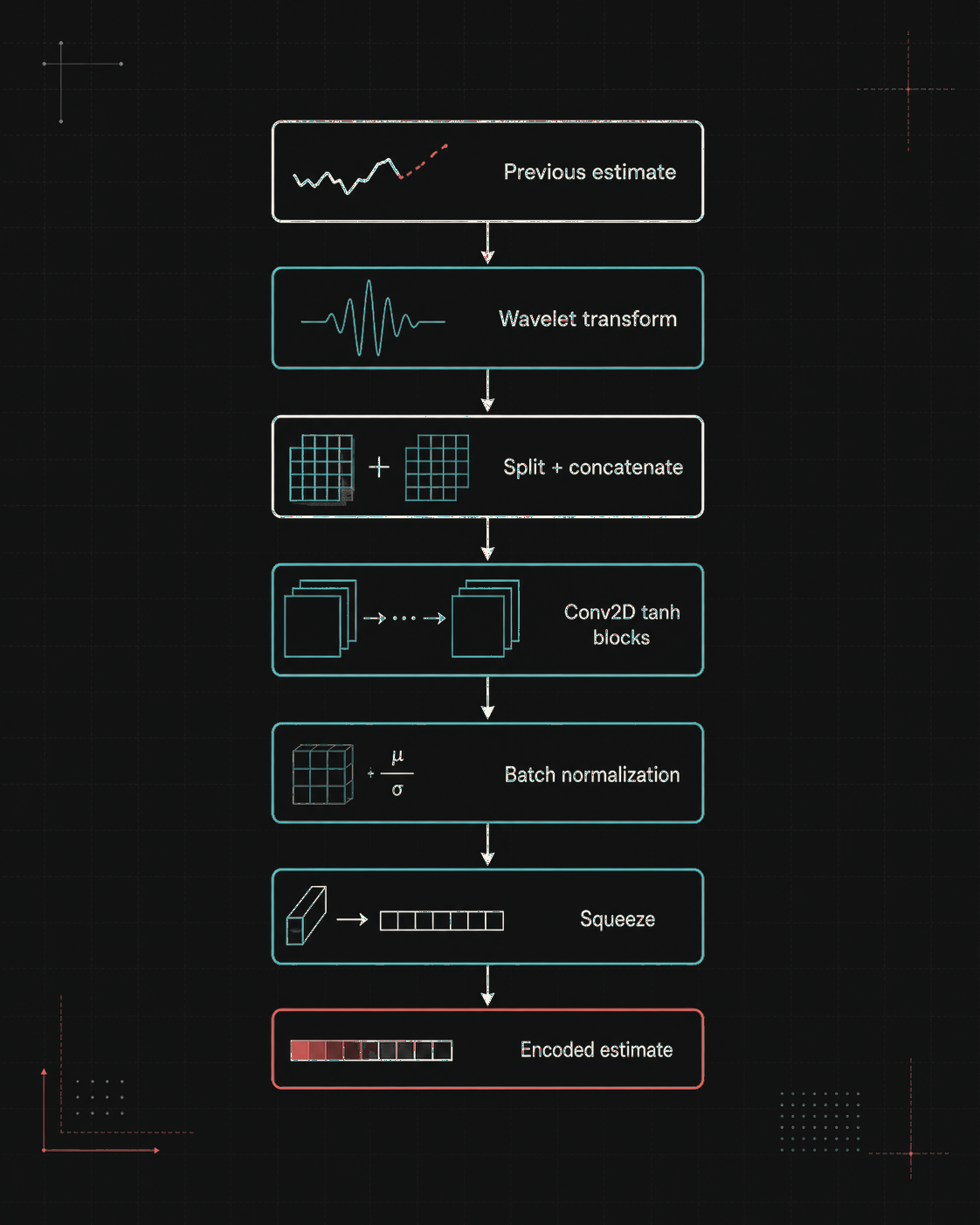
Per-layer filter and channel counts were fixed by the evaluated configuration in Figure 11 (window size 80, overlap 30, 30 subsamples) and follow the convolution–activation–batch-normalization block patterns described in Section 4 and the layer diagrams above.
Appendix B: Datasets
2021-2022 Bitcoin Dataset
Synthetic Dataset Sample
2018-2022 Bitcoin Dataset
Q4 2022 Validation Dataset
Bibliography
- Akram, M. A., Liu, P., Tahir, M. O., Ali, W., & Wang, Y. (2019). A state optimization model based on Kalman filtering and robust estimation theory for fusion of multi-source information in highly non-linear systems. Sensors, 19(7), 1687. https://doi.org/10.3390/s19071687
- Beale, M. H., Hagan, M. T., & Demuth, H. B. (2022). Deep Learning Toolbox Reference. MathWorks.
- Cai, W., Zhang, M., & Zhang, Y. (2017). Batch mode active learning for regression with expected model change. IEEE Transactions on Neural Networks and Learning Systems, 28(7), 1668–1681. https://doi.org/10.1109/tnnls.2016.2542184
- Ceravolo, R. (2004). Use of instantaneous estimators for the evaluation of structural damping. Journal of Sound and Vibration, 274(1–2), 385–401. https://doi.org/10.1016/j.jsv.2003.05.025
- Dahleh, M., Dahleh, M. A., & Verghese, G. (n.d.). Lectures on Dynamic Systems and Control. Massachusetts Institute of Technology, Department of Electrical Engineering and Computer Science.
- Emzir, M. F., Woolley, M. J., & Petersen, I. R. (n.d.). A Quantum Extended Kalman Filter. School of Engineering and IT, University of New South Wales. https://arxiv.org/abs/1603.01890
- Geerts, N. C. P. J. (1996). The Hilbert transform in complex Envelope Displacement Analysis (CEDA) (DCT rapporten, Vol. 1996.121). Technische Universiteit Eindhoven.
- Grover, R., & Hwang, P. Y. C. (2012). Introduction to Random Signals and Applied Kalman Filtering: With MATLAB Exercises. Wiley.
- Hommes, C. H. (2001). Financial markets as nonlinear adaptive evolutionary systems. Quantitative Finance, 1(1), 149–167. https://doi.org/10.1080/713665542
- Huber, P. J., & Ronchetti, E. M. (2011). Robust Statistics. Wiley.
- Hull, J. C. (2022). Options, Futures, and Other Derivatives. Pearson Education Limited.
- Isola, P., Zhu, J.-Y., Zhou, T., & Efros, A. A. (2018). Image-to-image translation with conditional adversarial networks. arXiv. https://arxiv.org/abs/1611.07004
- Kingma, D. P., & Ba, J. L. (2015). Adam: A method for stochastic optimization. ICLR. https://arxiv.org/abs/1412.6980
- Lee, T. K., Baddar, W. J., Kim, S. T., & Ro, Y. M. (2018). Convolution with logarithmic filter groups for efficient shallow CNN. MultiMedia Modeling, 117–129. https://doi.org/10.1007/978-3-319-73603-7_10
- Li, H., Mao, C. X., & Ou, J. P. (2013). Identification of hysteretic dynamic systems by using a hybrid extended Kalman filter and wavelet multiresolution analysis with limited observation. Journal of Engineering Mechanics, 139(5), 547–558. https://doi.org/10.1061/(asce)em.1943-7889.0000510
- Luna, J. (2022). Proposals for a Cryptocurrency Trading AI: Wavelets and Generative Adversarial Networks for Extrapolating Random Signals. Read on this site.
- Mili, L., Cheniae, M. G., Vichare, N. S., & Rousseeuw, P. J. (1996). Robust state estimation based on projection statistics of power systems. IEEE Transactions on Power Systems, 11(2), 1118–1127. https://doi.org/10.1109/59.496203
- Misiti, M., Misiti, Y., Oppenheim, G., & Poggi, J.-M. (2015). Wavelet Toolbox User's Guide. MathWorks.
- Peng, S. (2013). Design and Analysis of FIR Filters Based on MATLAB (thesis).
- Rankin, J. M. (1986). Kalman filtering approach to market price forecasting (Iowa State University Capstones, Theses and Dissertations). https://doi.org/10.31274/rtd-180813-7911
- Vaswani, A., Shazeer, N., Parmar, N., Uszkoreit, J., Jones, L., Gomez, A. N., Kaiser, Ł., & Polosukhin, I. (2017). Attention is all you need. 31st Conference on Neural Information Processing Systems (NeurIPS). https://arxiv.org/abs/1706.03762
- Williams, M. B. (2016). Fast Fourier Transform in Predicting Financial Securities Prices (thesis).
- Wu, N., Green, B., Ben, X., & O'Banion, S. (n.d.). Deep transformer models for time series forecasting: The influenza prevalence case. arXiv. https://arxiv.org/abs/2001.08317
- Zhang, C., & Huang, L. (n.d.). A Quantum Model for the Stock Market (thesis).
- Zhu, J.-Y., Park, T., Isola, P., & Efros, A. A. (2017). Unpaired image-to-image translation using cycle-consistent adversarial networks. 2017 IEEE International Conference on Computer Vision (ICCV). https://doi.org/10.1109/iccv.2017.244