Wavelet-Based Short-Horizon Forecasting of BTCUSDT Returns
Abstract
This report documents a MATLAB research prototype for short-horizon BTCUSDT return forecasting. The study compares raw-return inputs, wavelet-derived features, and a combined raw plus wavelet representation under matched baselines, ridge regression, and residual temporal convolutional networks. For the reported run, the central result is that wavelet-enhanced neural models do not outperform the simpler baselines: zero and mean forecasts win the main error metrics, ridge is strongest on directional accuracy and correlation, and raw TCN is only the best of the neural variants.
This is the controlled re-evaluation that closes the series. The premise was set out in the Trading AI Proposals, first built in the WaveGAN BTCUSDT Extrapolation Report, and specified in full in the Wavelet GAN Trading Prototype. Here the same intuition — that multiscale wavelet features should help short-horizon Bitcoin forecasting — is finally put on a fair, leakage-controlled benchmark, and the answer is sobering.
1. Introduction
WaveGAN-2 is a second-generation forecasting study built after the earlier WaveGAN project. Instead of learning a conditional mapping between wavelet-history tensors with a GAN, this iteration reframes the problem as direct multi-step forecasting of one-minute BTCUSDT returns and asks a narrower question: does wavelet preprocessing improve a controlled forecasting benchmark?
The project is intentionally conservative. It uses fixed chronological splits, train-only normalization, reproducible run metadata, and report-bundle artifacts tied to a specific experiment ID. That makes the result easier to trust, even when the answer is not flattering to the more complex models.
2. Research Question
The central question is whether a multiscale wavelet representation improves short-horizon return forecasts relative to raw-return inputs when the target, split logic, and evaluation metrics are all held constant.
2.1 Data and Target
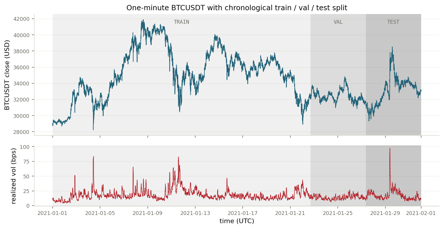
The reported run uses BTCUSDT 1-minute OHLCV data spanning January 1 through February 1, 2021. The supervised series is the one-minute log return, and the model target is the direct multi-step return path for horizons $H \in \{30, 60, 128\}$ with a fixed lookback window $L = 256$.
Windows are generated separately inside each chronological split so no sample crosses a train, validation, or test boundary. That prevents the leakage problems that often make financial forecasting experiments look better than they are.
2.2 Representations and Models
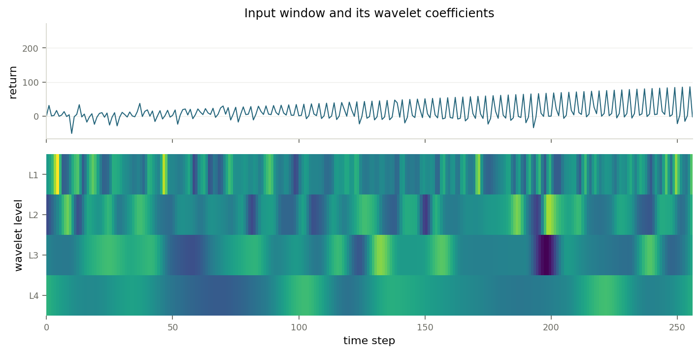
The pipeline compares three feature modes built from the same return windows: normalized raw returns, wavelet-derived features, and a combined raw plus wavelet representation. Those inputs are tested against simple baselines, a ridge comparator, and residual TCN models.
- Baselines: zero-return, last-return, and mean-return forecasts.
- Linear model: multivariate ridge regression on normalized raw windows.
- Neural models: raw TCN, wavelet TCN, and a dual-branch raw plus wavelet TCN.
3. Experimental Setup
The project is implemented as a config-driven MATLAB R2021b workflow. Each run saves config snapshots, figure bundles, metrics tables, model artifacts, and provenance metadata. Neural models are trained with Adam under a plain MSE objective after earlier mixed-loss variants showed unstable magnitude behavior.
3.1 Training and Evaluation
All models are scored in the original return domain using MAE, RMSE, stepwise directional accuracy, cumulative directional accuracy, and Pearson correlation. The default split is 70% train, 15% validation, and 15% test with no shuffle, and the reported neural seeds are 42, 43, and 44.
This framing matters because it turns the project into a matched comparison rather than a loose collection of plots. The simpler models and the neural models all face the same data, targets, and scoring rules.
3.2 Wavelet Provenance
One of the practical lessons from the project is that wavelet provenance cannot be hand-waved away. The pipeline records whether the preferred dual-tree complex wavelet path was used, whether a fallback was triggered, and how many dimensions the resulting feature vector contains.
For the reported run, saved metadata indicate the preferred DTCWT path with MATLAB's dualtree backend, no fallback, four decomposition levels, and 544-dimensional wavelet feature vectors at all three horizons.
4. Results
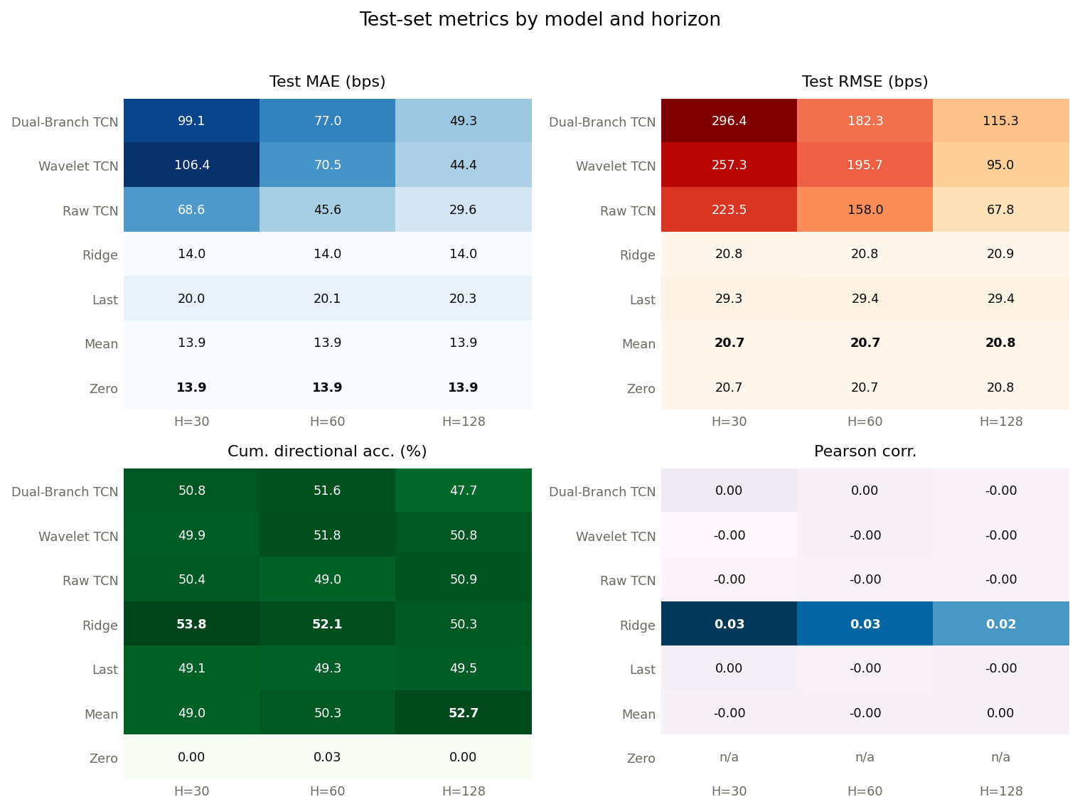
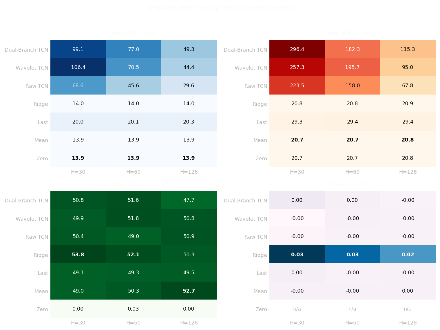
The main outcome is straightforward: wavelet-enhanced residual TCNs do not beat the simpler comparators in this setup. Zero and mean baselines are best on the primary error metrics, ridge is best on the nontrivial signal metrics, and raw TCN is only the strongest neural variant.
4.1 Main Comparison
| Model | H=30 MAE | H=60 MAE | H=128 MAE | H=30 Corr. | H=60 Corr. | H=128 Corr. |
|---|---|---|---|---|---|---|
| Zero | 13.88 bps | 13.89 bps | 13.91 bps | n/a | n/a | n/a |
| Mean | 13.88 bps | 13.89 bps | 13.91 bps | 0.000 | 0.000 | 0.000 |
| Last | 20.02 bps | 20.11 bps | 20.26 bps | 0.001 | -0.000 | -0.000 |
| Ridge | 13.96 bps | 13.98 bps | 14.02 bps | 0.033 | 0.026 | 0.019 |
| Raw TCN | 68.57 bps | 45.58 bps | 29.60 bps | -0.001 | -0.000 | -0.000 |
| Wavelet TCN | 106.43 bps | 70.52 bps | 44.43 bps | -0.002 | -0.000 | -0.000 |
| Dual-Branch TCN | 99.11 bps | 77.03 bps | 49.29 bps | 0.002 | 0.000 | -0.000 |
4.2 Horizon Examples
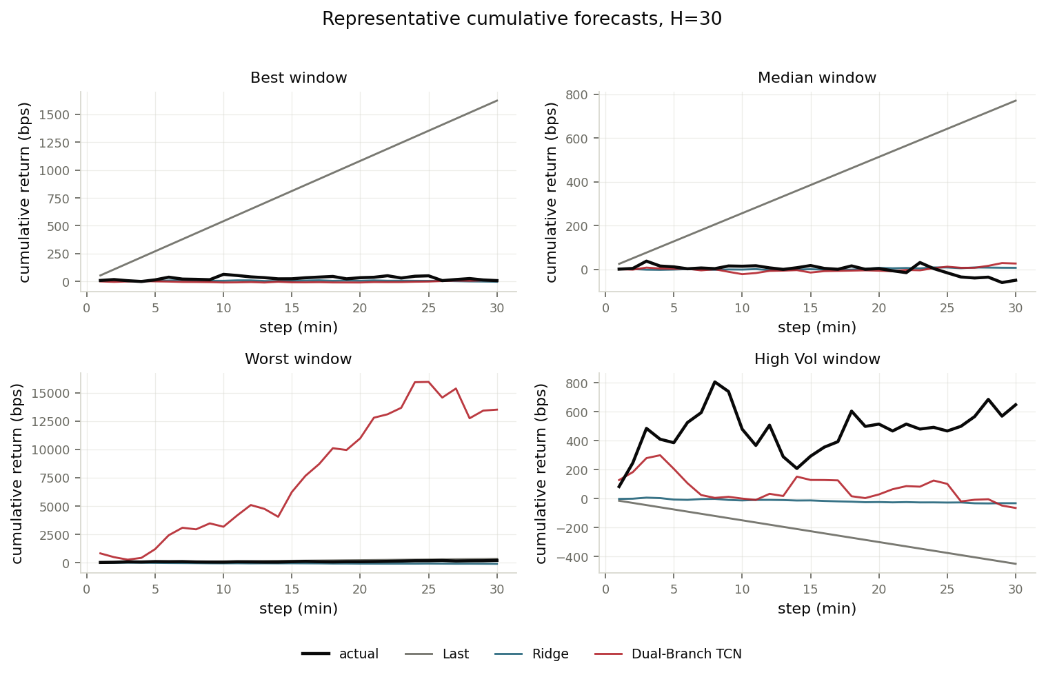
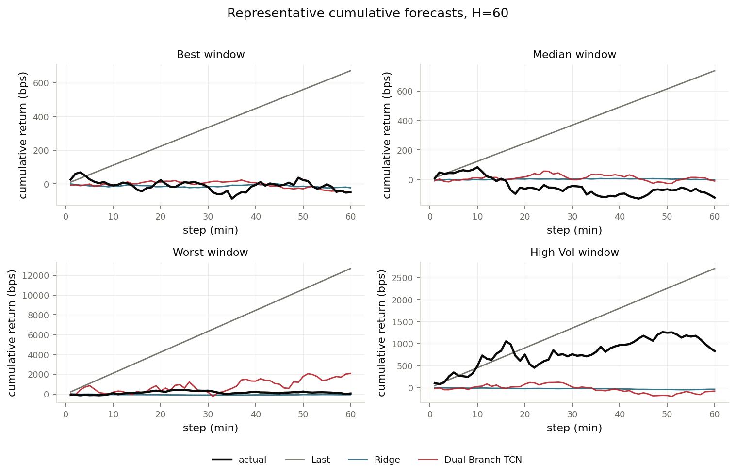
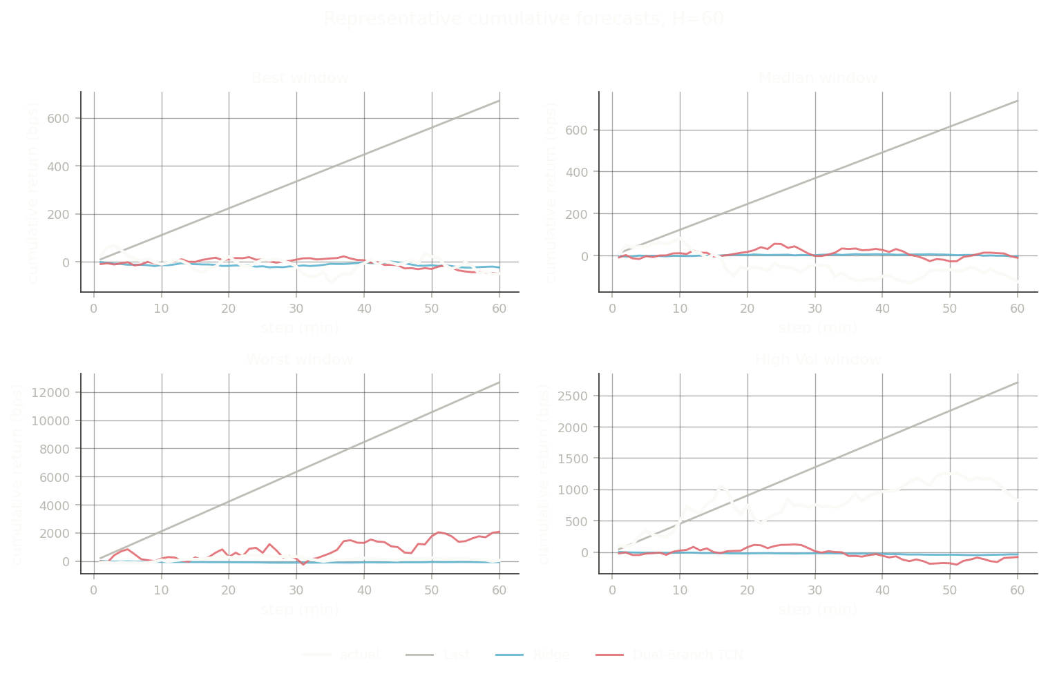
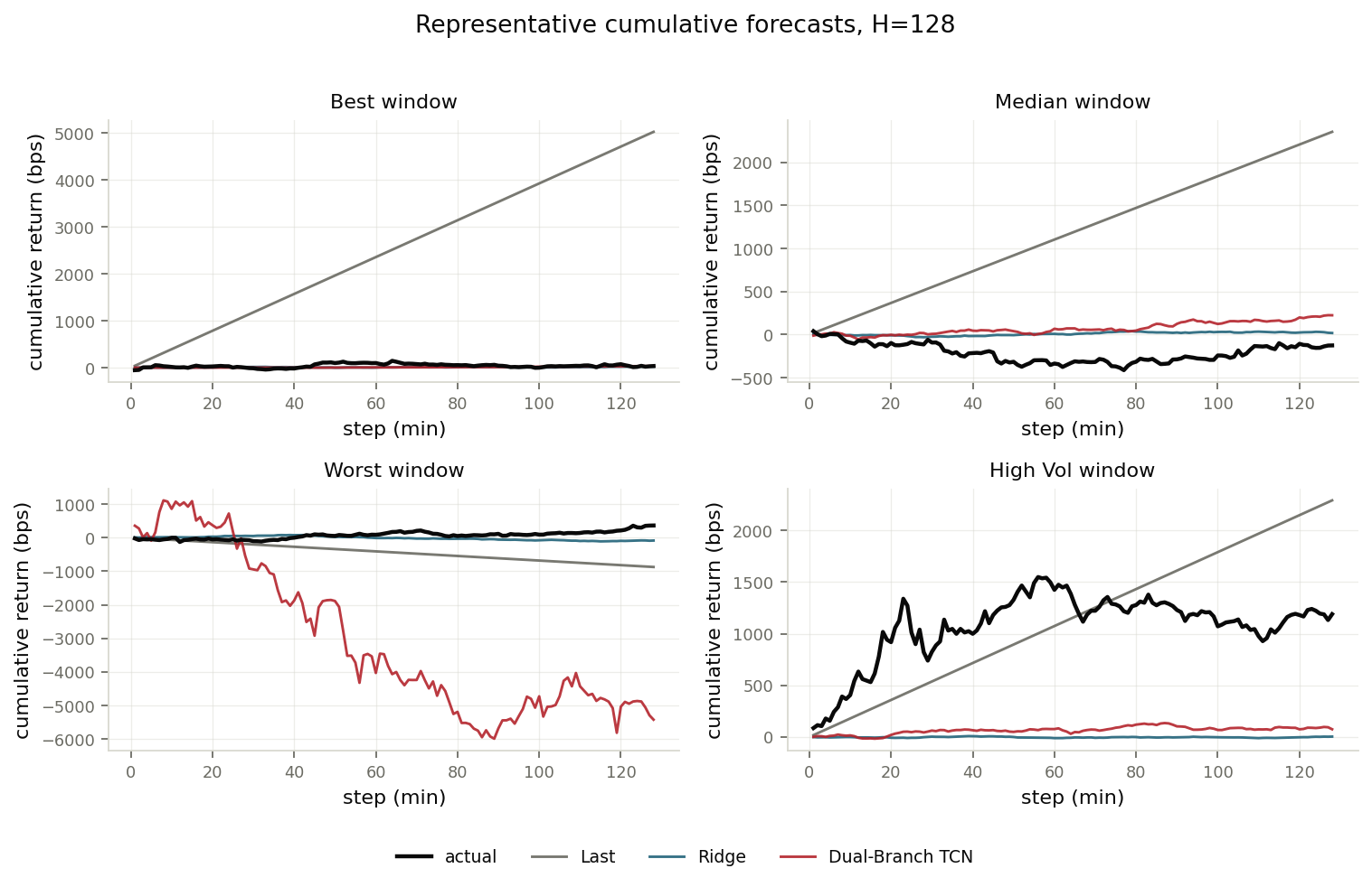
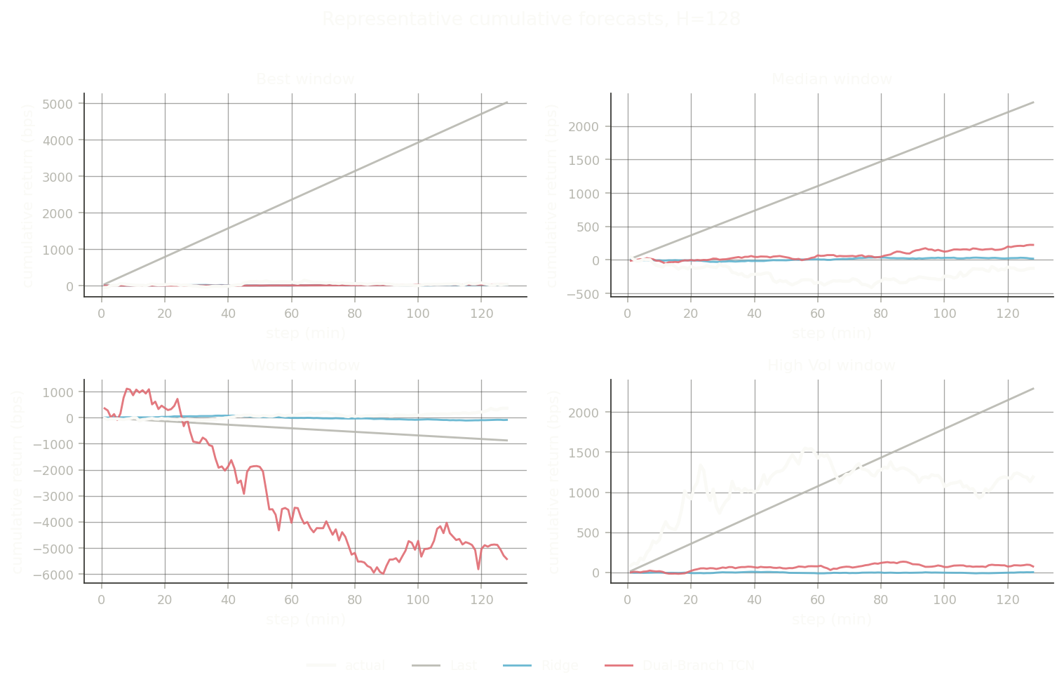
The representative forecast panels show that the neural models can track some benign windows, but reliability drops as the horizon grows. The $H=128$ case is where that weakness becomes the hardest to ignore.
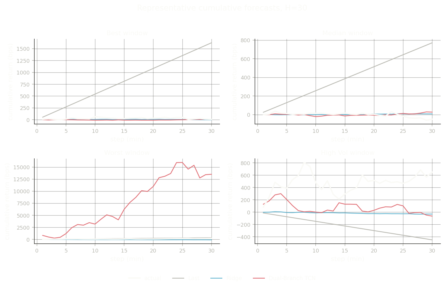
Each panel shows the actual cumulative return (black) against the predicted cumulative paths for the last-return baseline, ridge, and the dual-branch TCN, on a best, median, worst, and high-volatility window. The carry-forward baseline runs away from the actual path, and the dual-branch TCN destabilizes badly on the worst windows.
4.3 Aggregate Calibration
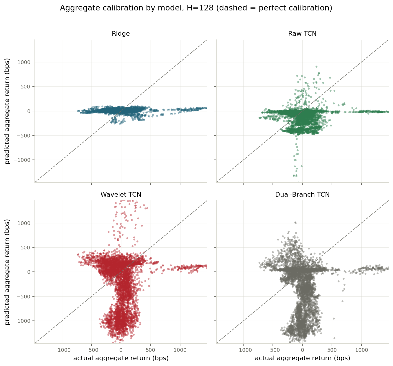
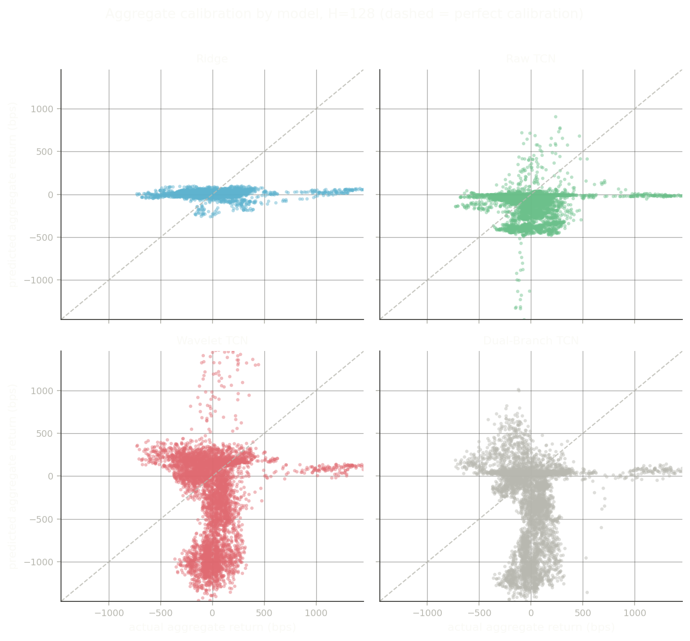
Aggregate calibration at $H=128$ reinforces the main result. Raw TCN captures a small amount of aggregate structure, but ridge remains better calibrated overall, and the wavelet-only and dual-branch models show poor slope and dispersion behavior on the harder horizon.
5. Interpretation
The main contribution of WaveGAN-2 is methodological clarity. The project takes a plausible intuition, that multiscale wavelet features should help short-horizon BTCUSDT forecasting, and subjects it to a controlled comparison that currently says no.
| Finding | Summary |
|---|---|
| Error metrics | Zero and mean baselines achieve the best MAE and RMSE at all three horizons, around 13.9 bps MAE. |
| Signal metrics | Ridge reaches the strongest directional accuracy and Pearson correlation, including 51.34% stepwise directional accuracy and 0.033 correlation at $H=30$. |
| Best neural model | Raw TCN is the strongest neural variant, but it remains materially worse than the simpler baselines on the primary error metrics. |
| Wavelet effect | Wavelet-only and dual-branch models are weaker than raw TCN, so the added wavelet representation does not help in the reported run. |
That is still progress. The MSE rollback removed the most unstable neural behavior seen in earlier prototypes, and the reporting pipeline now preserves enough provenance to make the next iteration more defensible. The next step is not more architectural ornament. It is better target design, better calibration, and richer covariates.
Read against the rest of the series, this is the honest endpoint of the arc that began with the Trading AI Proposals: the wavelet-and-GAN idea was coherent enough to build (WaveGAN) and specify in detail (the prototype), but once held to a fair, leakage-controlled benchmark it does not beat the simplest reasonable baselines. That is a useful result to have established cleanly.
6. Artifacts
- Read the full PDF report.
- Project stack: MATLAB R2021b, Deep Learning Toolbox, Wavelet Toolbox, optional Parallel Computing Toolbox.
- Reported run ID:
report_residual_tcn_mse_20260327_232949. - Saved outputs include config snapshots, metrics tables, report-bundle figures, model artifacts, and run metadata.