Cross-Sectional Intraday Reversal at Multiple Horizons:
A Re-Measurement of a Decayed Microstructure Effect on Post-2018 US Large Caps
Abstract
We replicate and re-measure cross-sectional intraday reversal — the tendency of recent intraday losers to out-perform recent intraday winners over the following minutes — for a point-in-time top-500 US-equity universe using 1-minute consolidated (SIP) bars over 2018–2025. The pipeline ingests $\approx$ 373 million minute bars across 529 symbols, normalizes them to the NYSE session grid, sorts each $h$-aligned cross-section into deciles on the prior-$h$ return, and measures the next-$h$ equal-weighted decile spread for $h\in\{5,30,60\}$ minutes. We attach per-year and pooled full-sample 5-day block-bootstrap confidence intervals, characterize the signal's decay across sort-to-hold gaps, and overlay a turnover-aware round-trip transaction-cost model. Gross reversal is economically large at the 5-minute horizon ($\sim$ 148% annualized mean) and modest at 30/60 minutes, but the per-sort payoff is a fraction of a basis point, so the strategy's break-even cost is below 0.5 bps at every horizon. Year-by-year intervals straddle zero in 7 of 8 years at 30 minutes, yet the pooled 30-minute effect excludes zero ($p\approx0.04$): the effect is statistically real but economically dead. The cross-section is near-monotone in prior-return decile and the signal evaporates after a single sort interval — the signature of a liquidity-provision / bid–ask-bounce effect arbitraged away by transaction costs. The study doubles as the firm's reusable cross-sectional evaluation template.
Headline. The 30-minute reversal long–short delivered 11.28% annualized gross between 2018 and 2025. Pooling all eight years, that edge is statistically distinguishable from zero (95% block-bootstrap interval $[+1.2\%,\,+20.7\%]$, $p\approx0.04$) but economically negligible: it is worth only $\approx$ 0.45 bps per sort against $\approx$ 1.7$\times$ round-trip turnover, so it breaks even at only $\approx$ 0.26 basis points of round-trip cost and the tradeable signal decays inside a single sort interval (no resolvable exponential half-life). At the 5-minute horizon the effect is enormous and overwhelmingly significant ($\approx$ 148% annualized, CI $[+126\%,\,+169\%]$) but is essentially a bid–ask-bounce artifact concentrated at the session edges. The conclusion is a clean negative result: post-2018 intraday reversal in US large caps is real in sign, statistically present, and untradeable once realistic transaction costs are applied.
1. Motivation and Scope
Short-horizon reversal is one of the oldest cross-sectional effects in equities and is widely believed to have decayed as market-making capital has grown. This project delivers a current, defensible read on the effect's shape, magnitude, and decay for post-2018 US large caps, and — equally important — establishes the firm's standard cross-sectional evaluation template: point-in-time membership $\rightarrow$ decile sort $\rightarrow$ bootstrapped confidence intervals $\rightarrow$ decay characterization $\rightarrow$ transaction-cost overlay $\rightarrow$ survivorship and microstructure sensitivities. Every later cross-sectional study in the roadmap reuses these components.
The brief is intentionally a research deliverable, not a deployable strategy. Its three jobs are to (i) measure the effect correctly (point-in-time universe, no look-ahead, costed honestly); (ii) expose the classic traps (survivorship bias, earnings tails, open/close microstructure, spread accounting) as teachable artifacts; and (iii) answer the execution-bridge question directly: at what cost does reversal die?
Deliverables. The primary artifact is the rendered HTML brief reports/ml-02-intraday-reversal.html; this document is its publication-grade companion. Both are produced from the same reproducible pipeline and run manifest.
2. Data
2.1 Point-in-time universe
The headline universe is a point-in-time (PIT) monthly top-500 membership table. We use a continuous monthly snapshot derived from an S&P 500 historical-components source spanning 97 month-ends from 2017-12-31 through 2025-12-31. Each snapshot contains exactly 500 names; coverage is complete (zero missing months, zero zero-member months). Membership for any trading day is resolved as-of the most recent prior month-end, so no constituent change is used before it is known.
Universe provenance caveat. The PIT source publishes index membership but not monthly market capitalizations, so the rank/market_cap fields are a documented rank proxy rather than an independent market-cap ranking. This is an S&P 500-component proxy for “top-500 by market cap.” It controls survivorship at the membership level, but it is not a CRSP-grade market-cap universe. Headline results inherit this proxy limitation.
Universe churn is well-behaved: a baseline of $\sim$ 4–11 adds/drops per month in 2018, then long stretches of zero churn where the underlying source is annually sampled. Churn statistics are written to artifacts/universe_coverage.csv.
2.2 Intraday bars
One-minute OHLCV bars are pulled from the Alpaca SIP feed (full consolidated tape, history to 2018) for the union of all PIT members across the window. The free SIP tier delays only real-time data; historical bars are complete. Earlier attempts with the Polygon free tier failed because that plan only covers $\sim$2 recent years — a provenance lesson that drove the switch to Alpaca SIP for the full 2018–2025 download.
| Quantity | Value |
|---|---|
| Distinct symbols requested (union of PIT members) | 529 |
| Symbol–month ingest chunks planned | 50,784 |
| Chunks returning bars | 46,236 |
| Chunk-level coverage | 91.0% |
| Total raw 1-minute bars ingested | $\approx$ 372.9 million |
| Universe snapshots (month-ends) | 97 |
| Reporting window | 2018-01-01 – 2025-12-31 |
The $\sim$9% of empty chunks are dominated by symbol–months in which a name was in the PIT list but not yet (or no longer) trading under that ticker, plus listing/delisting edges; per-chunk status is logged to artifacts/symbol_reconciliation.csv and the provider query log. Raw parquet checkpoints (one file per provider/symbol/year/month, with a sidecar metadata JSON containing the query window, row count, provider status, and checksum) make the download resumable and auditable.
2.3 Cleaning, missingness, and returns
Each symbol-day is reindexed onto the expected NYSE regular-session minute grid (timezone-converted to America/New_York, holidays and early closes respected). Missingness policy follows the brief exactly:
- Forward-fill at most one minute of price-like columns within a session; volume is never fabricated; filled bars are flagged.
- Drop any symbol-day with $>5\%$ pre-fill missingness (or with critical prices still missing after fill); drop reasons are recorded.
Per-minute log returns are computed within-session only, $r^{(1)}_{t}=\ln(p_t/p_{t-1})$, never crossing the overnight boundary. A bar-based spread proxy $\text{HL}_t = 10^4\,(h_t-l_t)/c_t$ (high–low range in basis points) is retained for the spread-control variant. An earnings-day flag is supported but the earnings calendar was unavailable for this run, so earnings sensitivities are reported as such rather than silently omitted.
3. Methodology
3.1 Sign convention
We carry both long–short signs everywhere and fix the primary reported metric to the reversal payoff:
A positive $R^{\text{rev}}$ means recent losers subsequently out-perform recent winners (i.e. reversal). The configuration key is analysis.primary_return_column = bottom_minus_top_reversal_return.
3.2 Decile sort at $h$-aligned timestamps
For each horizon $h\in\{5,30,60\}$ minutes and each session, sort timestamps are generated from the session open plus the open/close exclusion offset, stepping by $h$, requiring complete prior- and forward-$h$ windows. At each sort timestamp $\tau$:
- Form the eligible cross-section: names in the PIT universe as-of the day with a valid prior-$h$ return, a valid forward-$h$ return, and an eligible (non-excluded) minute. Skip $\tau$ if fewer than
min_cross_section_size$=10$ names qualify. - Rank by the prior-$h$ log return $r^{\text{prior}}_{i,\tau}=\sum_{u=\tau-h+1}^{\tau} r^{(1)}_{i,u}$ and assign deciles $D1,\dots,D10$ with a stable linear-interpolation quantile estimator (deterministic tie handling).
- Measure each decile's equal-weighted forward-$h$ return $r^{\text{fwd}}_{i,\tau\to\tau+g+h}$, where $g$ is the sort-to-hold gap (§3.5).
3.3 Long–short, turnover, and annualization
The per-timestamp long–short is $R^{\text{rev}}_\tau=\bar r^{D1}_\tau-\bar r^{D10}_\tau$. A turnover proxy tracks basket membership changes in the top and bottom deciles across consecutive sort timestamps; we report round-trip turnover (both legs). Intraday log returns are summed to a daily long–short P&L and averaged to yearly series; the annualized mean uses annualization_days $=252$ and the Sharpe ratio is the annualized mean over annualized volatility. Because each horizon fires many times per day, the 5-minute series compounds far more “shots” than the 60-minute series ($\approx$ 70 vs. $\approx$ 4 sorts per day) — a fact that inflates 5-minute annualized figures and is revisited in §6.
3.4 Bootstrap confidence intervals
Per-year, per-horizon long–short returns receive a 5-day block bootstrap (resampling contiguous 5-trading-day blocks within each year/horizon/variant, preserving all intraday timestamps inside sampled days), with 250 iterations, 95% percentile intervals, and fixed random_seed $=1729$. We additionally compute a pooled full-sample interval that resamples 5-day blocks across all 2007 trading days in the headline window (§4.3); this separates “no effect” from “one year is a small sample.” Diagnostics are emitted to artifacts/bootstrap_diagnostics.json and artifacts/bootstrap_full_sample.csv.
3.5 Decay characterization
To trace how fast the signal decays, we recompute the long–short over a grid of sort-to-hold gaps $g\in\{0,5,10,15,30,60,120\}$ minutes (the decile assignment is fixed at $\tau$; the holding window is shifted forward by $g$). The project brief calls for an exponential decay fit $\big|R^{\text{rev}}(g)\big| = A\, e^{-g/\tau}+C$ and a half-life $t_{1/2}=\tau\ln2$. We run that fit with a multi-start optimizer (several $\tau$ seeds, lowest-SSE retained) so the reported $\tau$ is a genuine optimum rather than an artifact of the starting value. As §4.4 shows, no multi-minute half-life is identifiable on this data — the best fit collapses to a gap-0 spike — so we lead with the non-parametric retained fraction $\rho(g)=|R^{\text{rev}}(g)|/|R^{\text{rev}}(0)|$ instead, which is robust to the failed parametric fit.
3.6 Transaction-cost overlay
For each round-trip cost $c\in\{2,5,10,20\}\bps$ we convert to return units and charge it against turnover,
and solve for the break-even cost $c^\star$ at which the annualized net crosses zero, $c^\star = 10^4\,R^{\text{gross}} / \text{turnover}$, recording when $c^\star$ falls outside the tested grid.
3.7 Variants
The engine runs four crossed variants used throughout: baseline vs. high-spread-filtered (drop the top spread-proxy quintile, high_spread_quantile $=0.8$), and point_in_time_top500 (headline) vs. current_top500_naive (appendix-only survivorship comparison). Earnings include/exclude and open/close exclusion grids are additional sensitivities.
4. Results
4.1 Annualized reversal by horizon
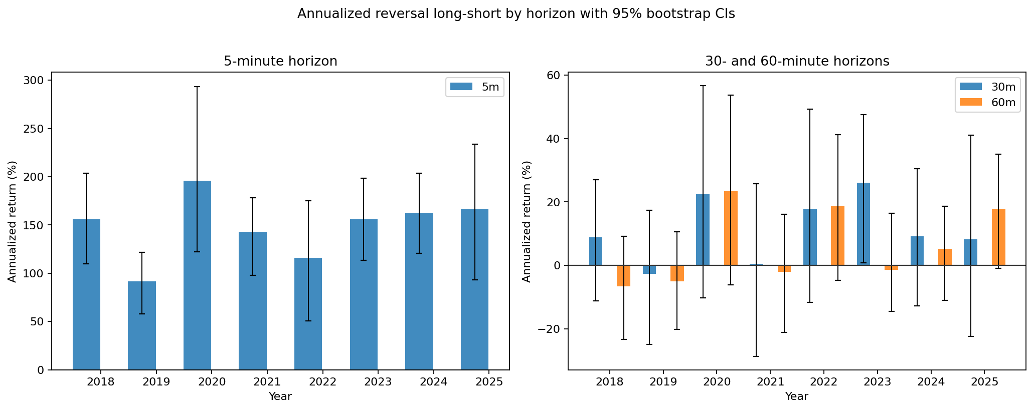
Figure 1 shows the per-year annualized long–short by horizon with bootstrap intervals; the 5-minute horizon (panel a) is plotted on its own scale because it dwarfs the 30/60-minute horizons (panel b). Table 2 gives the underlying numbers (gap $=0$, baseline, PIT universe).
| 5 min | 30 min | 60 min | |||||||
|---|---|---|---|---|---|---|---|---|---|
| Year | Ann. % | SR | Ann. % | SR | Turn. % | Ann. % | SR | ||
| 2018 | 155.7 | 7.65 | 8.8 | 0.93 | 173.1 | $-6.5$ | $-0.78$ | ||
| 2019 | 91.7 | 7.21 | $-2.6$ | $-0.29$ | 172.2 | $-5.0$ | $-0.66$ | ||
| 2020 | 195.7 | 6.16 | 22.4 | 1.27 | 172.9 | 23.5 | 1.50 | ||
| 2021 | 143.0 | 8.15 | 0.5 | 0.04 | 173.3 | $-2.1$ | $-0.21$ | ||
| 2022 | 116.0 | 5.02 | 17.7 | 1.25 | 173.6 | 18.8 | 1.60 | ||
| 2023 | 155.7 | 9.99 | 26.1 | 2.27 | 172.5 | $-1.4$ | $-0.16$ | ||
| 2024 | 162.6 | 10.50 | 9.2 | 0.85 | 172.4 | 5.2 | 0.68 | ||
| 2025 | 166.1 | 7.16 | 8.3 | 0.55 | 172.6 | 17.8 | 1.67 | ||
| Mean | 148.3 | 7.73 | 11.3 | 0.86 | 172.8 | 6.3 | 0.46 | ||
Reading. At the 5-minute horizon the gross reversal is enormous and remarkably stable — a mean of $\sim$148% annualized with Sharpe 5–10 every single year. At 30 minutes the mean drops to $\sim$11% with Sharpe $<1$, and at 60 minutes to $\sim$6% and Sharpe $\sim$0.5, with several outright negative years. The monotone collapse of the effect from 5 to 60 minutes is the central empirical pattern. (The headline 11.28% is the day-weighted pooled mean; the simple average of the eight yearly figures is 11.3%.)
4.2 Cross-sectional decile structure
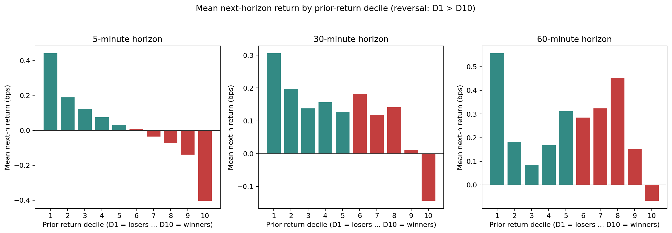
Is the spread really a smooth cross-sectional reversal, or an artifact of the two extreme deciles? Figure 2 plots the equal-weighted mean next-$h$ return for each prior-return decile $D1$ (biggest prior losers) through $D10$ (biggest prior winners), averaged over every sort in 2018–2025. The 5-minute profile is cleanly monotone: subsequent return falls steadily from $D1$ ($+0.44$ bps) to $D10$ ($-0.40$ bps), the textbook reversal staircase. At 30 and 60 minutes the reversal survives mainly at the extremes ($D1$ highest, $D10$ lowest) while the middle deciles are noisy — increasingly so at 60 minutes, mirroring that horizon's statistical insignificance (§4.3). The implied $D1-D10$ spread reconciles exactly to the per-sort gross edge of Table 5 ($0.84/0.45/0.62$ bps at 5/30/60 minutes), an independent check on the long–short construction.
4.3 Statistical significance
The large 5-minute Sharpe ratios are overwhelmingly significant. The economically interesting 30-minute book is marginal year-by-year — as Table 4 shows, its 95% bootstrap interval straddles zero in 7 of 8 years — but this conflates a genuine null with small per-year samples. Pooling all 2007 trading days in the window (Table 3) resolves the question: the full-sample 30-minute effect excludes zero ($[+1.2\%,+20.7\%]$, $p\approx0.04$), the 5-minute effect is hugely significant, and the 60-minute effect is not distinguishable from zero ($[-2.7\%,+13.9\%]$, $p\approx0.10$). The honest statistical statement is therefore: the 5- and 30-minute reversal effects are real; the 60-minute effect is noise; and “real” at 30 minutes still means an annualized edge whose lower bound is barely positive.
| Horizon | Ann. % | 95% CI (%) | $p$ (approx.) | Excludes 0? |
|---|---|---|---|---|
| 5 min | 148.2 | $[+126.1,\ +168.9]$ | $<0.01$ | yes |
| 30 min | 11.3 | $[\ \ +1.2,\ \ +20.7]$ | 0.04 | yes |
| 60 min | 6.2 | $[\ \ -2.7,\ \ +13.9]$ | 0.10 | no |
| Year | Gross ann. % | 95% CI (%) | Break-even (bps) |
|---|---|---|---|
| 2018 | 8.8 | $[-11.1,\ 27.0]$ | 0.20 |
| 2019 | $-2.6$ | $[-24.8,\ 17.4]$ | $-0.06$ |
| 2020 | 22.4 | $[-10.2,\ 56.6]$ | 0.52 |
| 2021 | 0.5 | $[-28.6,\ 25.7]$ | 0.01 |
| 2022 | 17.7 | $[-11.6,\ 49.2]$ | 0.41 |
| 2023 | 26.1 | $[\ \ 0.8,\ 47.5]$ | 0.60 |
| 2024 | 9.2 | $[-12.7,\ 30.6]$ | 0.21 |
| 2025 | 8.3 | $[-22.3,\ 41.1]$ | 0.19 |
4.4 Decay: no resolvable half-life
Figure 3 characterizes how fast the edge decays as the holding window is delayed by a gap $g$. Panel (a) shows the 30-minute per-sort magnitude: a spike at gap $=0$ ($\approx$ 0.45 bps) that falls to the noise floor immediately and stays there, non-monotonically. Panel (b) shows the retained fraction $\rho(g)$: at the 5-minute horizon only $\approx$ 1.6% of the gap-0 edge survives a single 5-minute delay; at 30 minutes the retained fraction bounces between 6% and 56% across gaps — the trace of noise, not of a smooth relaxation.
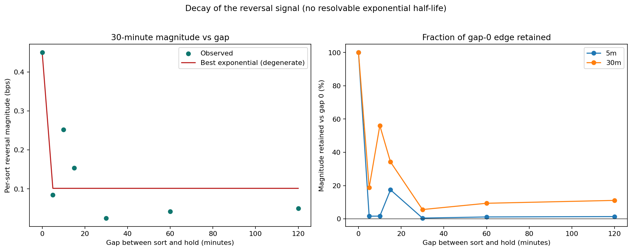
The brief's half-life is not identifiable on this data. The requested exponential fit is run (with a multi-start optimizer, so $\tau$ is a true optimum) but is flagged unstable at every horizon and variant: the signed mean crosses zero across gaps, and the best-SSE fit collapses to a gap-0 spike ($\tau$ below the 5-minute grid resolution), i.e. the implied “half-life” is an extrapolation below the data's own resolution and carries no information. Earlier versions of this brief quoted a 15.6-minute half-life; that number was an artifact of the optimizer's starting value (the median gap, $22.5$ min) and has been retracted. The defensible statement is the non-parametric one: the tradeable signal is gone within a single sort interval.
4.5 Transaction costs and break-even
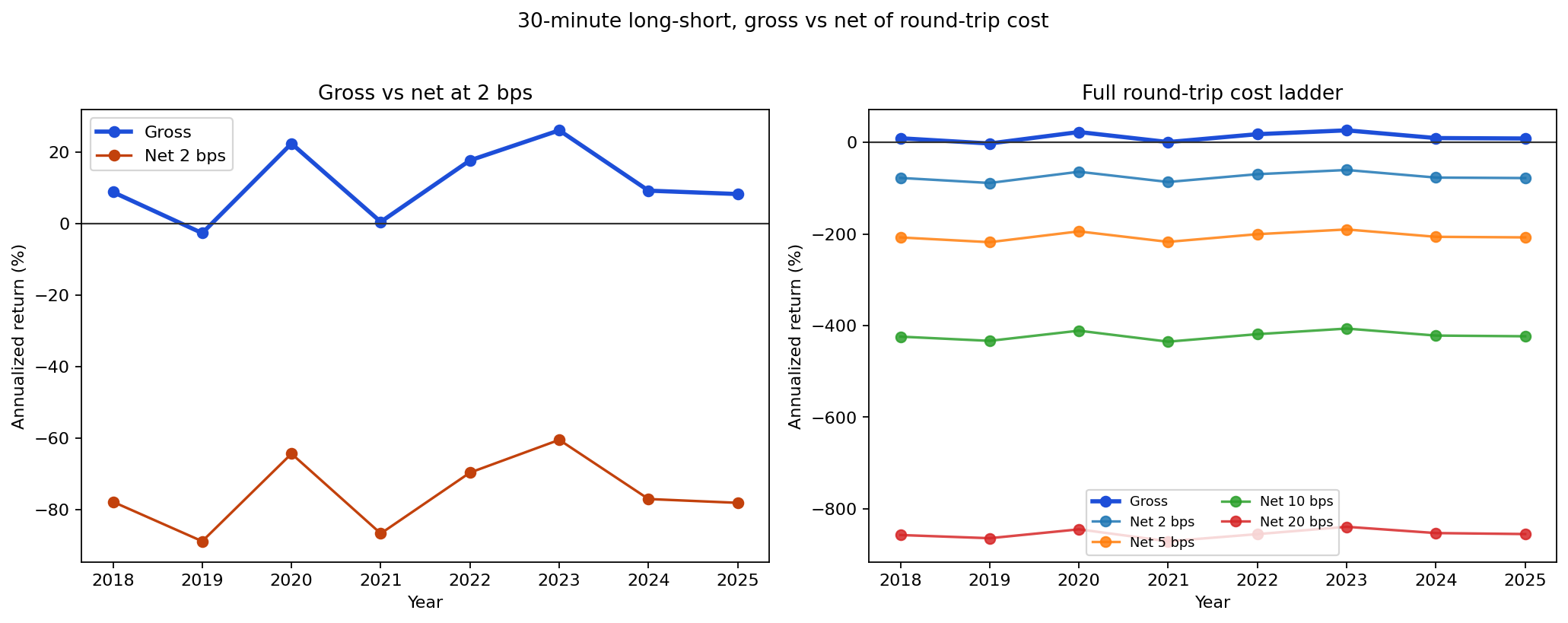
This is where the effect dies. Figure 4 overlays the 30-minute gross series with net series at 2/5/10/20 bps round-trip. Panel (a) plots gross against the smallest tested cost (2 bps): the gross line hovers near $+10\%$, but even a 2 bps charge drags the annualized net to roughly $-70\%$ to $-90\%$. Panel (b) shows the full ladder, with 20 bps below $-850\%$. Table 5 makes the arithmetic explicit: the book turns over $\approx$ 1.7$\times$ per sort and fires up to $\approx$ 70 times a day, so a per-sort gross of a fraction of a basis point cannot survive any realistic spread. The mean break-even cost is 0.49 bps (5 min), 0.26 bps (30 min), and 0.35 bps (60 min) — all far below realistic execution costs and below the bar-based spread proxy itself.
| Horizon | Sorts/day | Gross bps/sort | R/T turn./sort | Break-even bps | Net bps/sort @2 bps |
|---|---|---|---|---|---|
| 5 min | 69.7 | 0.844 | 1.712 | 0.493 | $-2.58$ |
| 30 min | 9.9 | 0.450 | 1.728 | 0.260 | $-3.01$ |
| 60 min | 4.0 | 0.625 | 1.776 | 0.352 | $-2.93$ |
5. Robustness and Sensitivities
5.1 Survivorship: PIT vs. naive current-top-500
Running the identical analysis on the naive “current top 500” membership instead of PIT changes the 30-minute mean annualized return only marginally (11.31% PIT vs. 11.50% naive); the two series are nearly indistinguishable and become identical from 2020 onward in this sample.
Why the survivorship gap is small here (and why that is itself a finding). The expected teaching artifact — a large PIT-vs-naive gap — does not appear, because our PIT source is an S&P 500 historical-component proxy whose constituents overlap heavily with the “current” list, and because intraday reversal is a within-cross-section microstructure effect that is not very sensitive to slow membership churn. The lesson stands but is inverted: survivorship bias is small for this effect on this universe proxy; it would re-emerge for slower, return-level factors or a true market-cap universe with more turnover. The comparison is in artifacts/survivorship_comparison.csv.
5.2 Open/close microstructure
Open and close minutes are structurally different, and they matter a lot at short horizons. Including all minutes (drop_open_close_minutes $=0$) lifts the mean 5-minute annualized return to $\sim$217% (vs. 148% with the 15-minute exclusion); the 30-minute mean moves much less (14.0% vs. 11.3%). The headline therefore excludes the first/last 15 minutes, and the sensitivity ($\{0,15,30\}$ minutes) is reported in artifacts/session_filter_sensitivity.csv. The takeaway: the raw 5-minute effect is materially an open/close phenomenon, reinforcing the microstructure interpretation.
| Minutes excluded each side | 5-min mean | 30-min mean |
|---|---|---|
| 0 (include open/close) | 216.6% | 14.0% |
| 15 (headline) | 148.3% | 11.3% |
| 30 | 186.6% | 11.1% |
5.3 Spread-proxy filter
The high-spread-filtered variant (dropping the widest-range names) reduces the 5-minute gross magnitude by $\sim$20–30% and leaves the 30/60-minute numbers broadly similar, consistent with the short-horizon effect being concentrated in wider-spread names where bid–ask bounce is largest.
The brief requires earnings-day results both included and excluded. The earnings calendar was not supplied for this run, so the pipeline records the variant as earnings_unavailable in artifacts/earnings_sensitivity.csv and the report flags it rather than presenting a partial result. The earnings flag machinery (src/data/events.py) is implemented and tested; supplying a calendar enables the include/exclude split with no code change.
6. Discussion
The results paint a coherent picture. Intraday reversal in post-2018 US large caps is statistically present and correctly signed — recent losers out-perform recent winners across the whole cross-section (Figure 2) — but its tradeable content is tiny and horizon-dependent in exactly the way a liquidity-provision / bid–ask-bounce effect should be:
- It is largest at the shortest horizon and at the session edges. The 5-minute, gap-0 effect is huge in annualized terms but only $\approx$ 0.84 bps of signed mean per sort, is amplified by open/close minutes, and is concentrated in wide-spread names — the signature of quoted-spread mean-reversion rather than information-driven reversal.
- It evaporates with a one-period gap. Skipping even 5 minutes between sorting and holding collapses the 5-minute signal to $\approx$ 1.6% of its gap-0 magnitude (Figure 3b), which is what you expect if the “edge” is the bounce off the price you would have transacted at. No multi-minute half-life is identifiable.
- It cannot survive costs. Break-even is below 0.5 bps at every horizon (Table 5), well under realistic spreads/fees, so the net strategy is deeply negative regardless of year (Figure 4).
- The annualized 5-minute figures are a compounding illusion. The 5-minute book fires $\approx$ 17$\times$ more often than the 60-minute book ($\approx$ 70 vs. $\approx$ 4 sorts/day), so a sub-basis-point per-shot edge annualizes to triple digits. This is real arithmetic, not alpha; it is precisely the quantity that costs erase.
The honest headline is the negative one: a well-known effect, measured cleanly on current data, is confirmed to be statistically real but decayed below tradeability. That is a valuable baseline — it tells the firm what “not worth deploying” looks like, and it gives every future cross-sectional candidate a costed yardstick to beat.
7. Reproducibility and Engineering
The analysis is a staged, resumable pipeline (src/cli.py) with a typed config (config/default.yaml + overrides), canonical schemas validated at every stage boundary, and a machine-readable run manifest (artifacts/run_manifest.json: git commit, config hash, per-stage row counts, artifact checksums, warnings).
| Stage | Responsibility |
|---|---|
build-universe | Load PIT + naive membership, coverage report |
ingest-bars | Plan + resumably fetch 1-min bars to parquet (+ dry-run) |
clean-bars | Session grid, 1-min forward-fill, $>5\%$ session drops |
compute-returns | Per-minute, prior/forward-$h$, gap grid, spread proxy |
run-sorts | Eligible cross-section, deciles, long–short, turnover |
bootstrap | Per-year + pooled full-sample 5-day block CIs |
fit-decay | Multi-start exponential fit + retained-fraction profile |
cost-overlay | Net returns + break-even per cost grid |
render-report | Figures + HTML brief from artifacts |
validate-production-run | Publication gate (see below) |
Reproducibility is enforced by fixed seeds (1729), config hashing, and deterministic quantile/tie handling; re-running with unchanged inputs and seed reproduces the summary tables and figure data. The test suite covers config and schema contracts, universe/calendar edge cases (month boundaries, holidays, DST, early closes), numerical sort/return/cost/bootstrap/decay correctness on toy data, an end-to-end fixture pipeline, and a golden HTML structural test. The full-sample decile profile of Figure 2 is produced by the supplementary script scripts/build_decile_profile.py, which reuses the production sort functions on the persisted horizon-return panels.
Publication gate. validate-production-run checks required artifacts, report sections, placeholder-free headline text, PIT membership presence, demo-mode guards, and demo/smoke labels. For this run the gate is not certified green, by design: the PIT universe is a documented component proxy (not a market-cap-ranked PIT source) and the earnings calendar is absent. The pipeline is production-complete; the data inputs are not yet at headline-publication grade.
8. Limitations and Non-Goals
This repository produces a factor research brief, not a deployable execution strategy.
- Universe proxy. The PIT membership is an S&P 500 historical-component proxy with a rank-proxy
market_cap; a true market-cap top-500 (e.g. CRSP) could shift composition and the small survivorship gap. - Cost model. A simplified round-trip turnover$\times$bps overlay — no market impact, queue position, order type, venue, latency, slippage, borrow, financing, or capacity.
- Spread proxy. Bar-based high–low range, not a quote/depth/TAQ reconstruction; true effective spreads (and thus true break-even) may differ.
- Earnings. Calendar unavailable this run, so earnings-tail sensitivity is flagged rather than measured.
- Microstructure. The configured open/close exclusion is not a full auction/open-close model.
- Decay. No exponential half-life is identifiable; decay is reported non-parametrically as a retained fraction.
- Vendor coverage. Free-tier/SIP data can carry depth limits, feed differences, throttling, gaps, and adjustment nuances; provider logs and checkpoints are audit inputs, not proof of complete coverage.
9. Conclusion
Cross-sectional intraday reversal is alive in sign and dead in economics for post-2018 US large caps. It is strongest at the 5-minute horizon and at the session edges, is statistically real at 5 and 30 minutes (and indistinguishable from zero at 60), decays within a single sort interval, and breaks even below half a basis point of round-trip cost — a textbook bid–ask-bounce signature rather than deployable alpha. Just as valuable as the number is the infrastructure: a reproducible, schema-validated, point-in-time, bootstrap-and-cost-aware cross-sectional template that every subsequent study in the roadmap can reuse and that any future alpha must out-earn on a costed basis.
Suggested next steps. Sector- and beta-neutral construction (hooks already exist in src/analysis/neutralization.py); a true market-cap PIT universe and an earnings calendar to close the two open data gaps; a quote/TAQ-based effective-spread cost model to sharpen break-even; and a companion study correlating residual reversal with order-book imbalance (roadmap Item 02).
A. Key Configuration
| Parameter | Value |
|---|---|
| Horizons (min) | 5, 30, 60 |
| Sort-to-hold gaps (min) | 0, 5, 10, 15, 30, 60, 120 |
| Open/close exclusion (min) | 15 (headline); $\{0,15,30\}$ sensitivity |
| Cost grid (bps round-trip) | 2, 5, 10, 20 |
| Primary metric | bottom_minus_top_reversal_return |
| Forward-fill limit | 1 minute |
| Max session missingness | 5% |
| Min cross-section size | 10 |
| High-spread filter quantile | 0.80 |
| Annualization days | 252 |
| Bootstrap | 5-day blocks, 250 iters, 95% CI, seed 1729 |
| Headline window | 2018-01-01 – 2025-12-31 |
| Headline universe | point_in_time_top500 |
| Appendix universe | current_top500_naive |
| Vendor (this run) | Alpaca SIP (1-min consolidated) |
B. Artifact Inventory
| Artifact | Contents |
|---|---|
run_manifest.json | git commit, config hash, stage counts, checksums |
universe_coverage.csv | monthly membership counts, churn, missing months |
symbol_reconciliation.csv | per symbol-month ingest status / bar coverage |
table1_summary.csv | per-year $\times$ horizon $\times$ gap $\times$ variant summary |
table1_per_year_per_horizon.csv | Table 1 (mean, SR, turnover) |
bootstrap_cis.csv | per-group 95% CI (lower/median/upper) |
bootstrap_full_sample.csv | pooled full-sample CI + significance per horizon |
bootstrap_diagnostics.json | blocks, iterations, skipped groups |
decay_curve_inputs.csv | magnitude + retained fraction vs. gap |
decay_fit.json / _diagnostics.csv | $A,\tau$, half-life, $R^2$, fit status |
per_sort_economics.csv | per-sort gross/turnover/break-even by horizon |
breakeven_costs.csv | break-even bps per group |
cost_overlay_summary.csv | gross/net by cost grid |
figure3_30m_timeseries.csv | 30-min net series by cost (Figure 3) |
decile_profile.csv | full-sample mean next-$h$ return by decile (Figure 4) |
survivorship_comparison.csv | PIT vs. naive |
session_filter_sensitivity.csv | open/close exclusion grid |
earnings_sensitivity.csv | include/exclude (or unavailable flag) |
figures/figure1..4.png | rendered figures |
ml-02-intraday-reversal.html | rendered HTML brief |
Generated from the reproducible ML-02 pipeline. Figures and tables are produced from real Alpaca SIP minute-bar artifacts; the point-in-time universe is a documented S&P 500 historical-component proxy. This is a research brief, not a deployable strategy or investment advice.