Order-Book Imbalance as a One-Second Predictor
Abstract
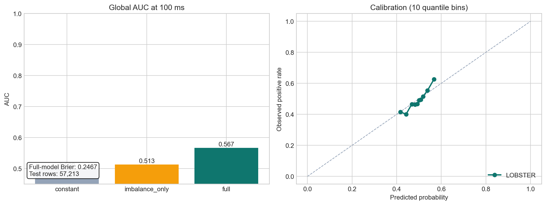
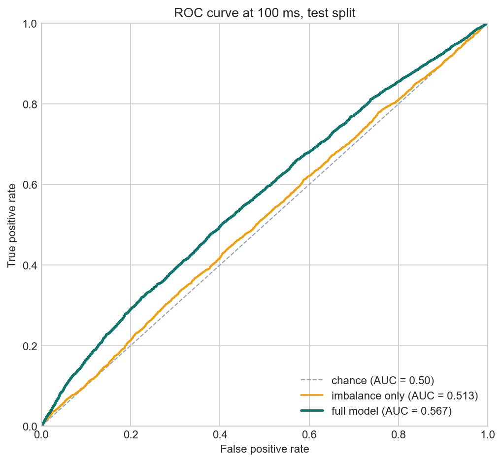
We evaluate whether top-five order-book imbalance, top-of-book spread, and prior-one-second signed trade imbalance predict the direction of the next mid-price move one second ahead on a single, fully-reproducible LOBSTER trading day. The result is a clean, auditable execution-research baseline rather than a profitability claim: on LOBSTER AAPL for 2012-06-21, sampled at 100 ms, the full logistic specification attains held-out ROC AUC $0.567$ and Brier score $0.2467$ on a chronologically-split test window covering 12:28:16–15:59:58 (eight 30-minute time-of-day buckets, 57,213 observations, 36 distinct spread tick values). After a taker-style cost overlay (full spread crossing plus a 1 bp fee), the strategy delivers net expected value of $-\$0.048$ per snapshot at the primary $0.55$ decision threshold ($-\$0.167$ per action across $16{,}584$ actions, $71\%$ no-trade share), so the signal does not survive realistic transaction costs in this single-day sample. Within the model, the prior-one-second signed-trade-imbalance coefficient carries the largest standardized magnitude (and a negative sign, consistent with short-horizon mean reversion), while top-five depth imbalance contributes a smaller positive coefficient.
1. Methodology Box
| Field | Specification |
|---|---|
| Data | LOBSTER sample for AAPL on 2012-06-21 (event file + 10-level orderbook CSVs). |
| Reconstruction | Event-time top-five book states normalized into a venue-agnostic canonical schema, then sampled backward without lookahead. |
| Features | Top-five signed depth imbalance $I_t^{(5)}$, top-of-book spread in ticks, prior-one-second signed-trade imbalance, 30-minute time-of-day bucket. |
| Label | $y_t = \mathbf{1}\{\Delta_h m_t > 0\}$ for horizon $h = 1$ s, computed as the first sampled mid-price at or after $t+h$; no-change ties dropped and counted. |
| Model | Logistic regression with $\ell_2$ regularization, fit on standardized features via L-BFGS-B; compared against constant base-rate and imbalance-only baselines. |
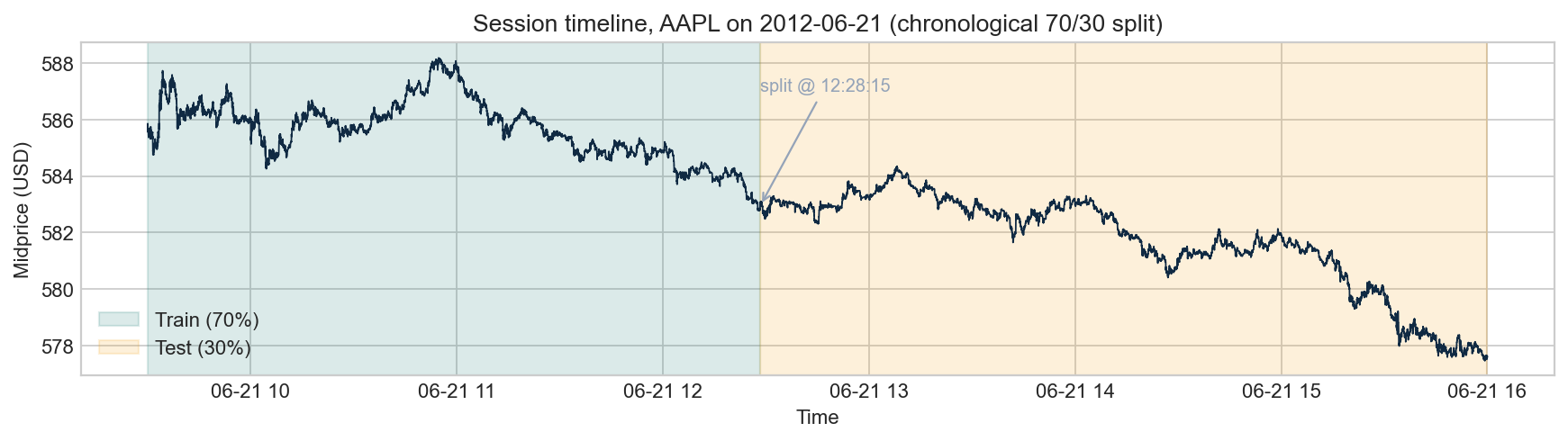
| Split | Chronological 70/30 (no shuffling); train $\le$ 12:28:15, test $\ge$ 12:28:16. |
| Evaluation | Global ROC AUC + Brier; calibration (10 quantile bins); AUC by 30-minute TOD bucket; AUC by spread quintile (per-venue boundaries); cadence ablations at 50/100/250 ms. |
| Cost assumptions | Taker-style full-spread crossing plus a 1 bp taker fee on notional; threshold sweep $\{0.50,0.55,0.60\}$; cost-multiplier sweep $\{0.5,1.0,1.5\}\times$. |
| Reproducibility | python -m src.cli run-all --source raw on the raw CSVs placed under data/raw/lobster/. |
2. Data and Reconstruction
The raw inputs are a LOBSTER event file and a matching 10-level order-book file for AAPL on 2012-06-21. Message events are joined to their corresponding orderbook row by position; the orderbook file is treated as authoritative for top-five state after each event. The pipeline writes one canonical event-book output per cadence for downstream modeling and reporting.
Data appendix.
- Session window: 09:30:00.004 – 15:59:59.913 (6.5 hours).
- Event-book rows: 400,391 raw events.
- Trades extracted: 34,990; aggressor-flagged share: 100% (no tick-rule inference required on this sample because every trade carries an explicit aggressor flag).
- Duplicate sub-millisecond timestamps: 16,062 (kept; the cadence sampler uses backward-fill with a 1 s staleness guard so duplicates do not corrupt the snapshot stream).
- Crossed books, non-monotonic levels, non-positive sizes, missing levels: all zero.
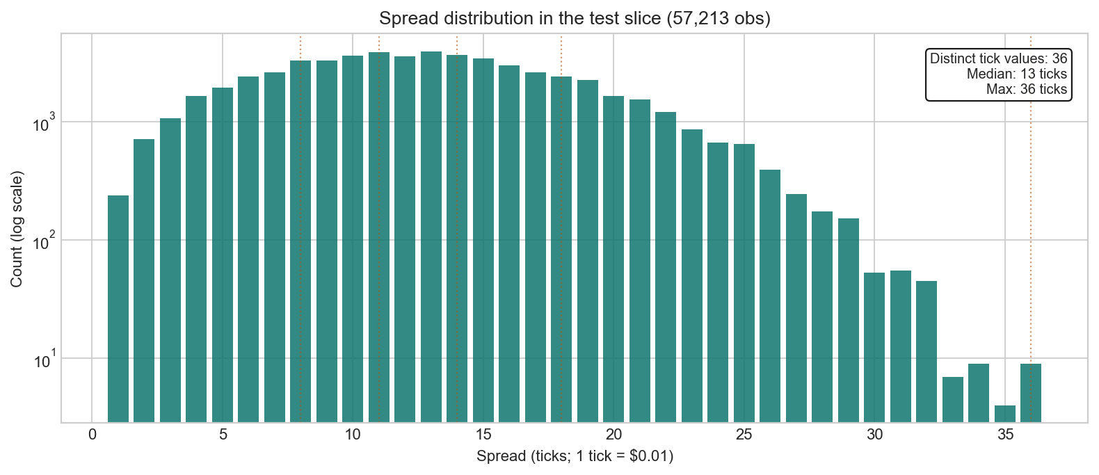
- Spread distribution in the held-out slice: 36 distinct tick values, median 13 ticks, max 36 ticks (Figure 7). Spread quintile boundaries are non-degenerate, so the stratified spread analysis rests on a genuinely varied distribution.
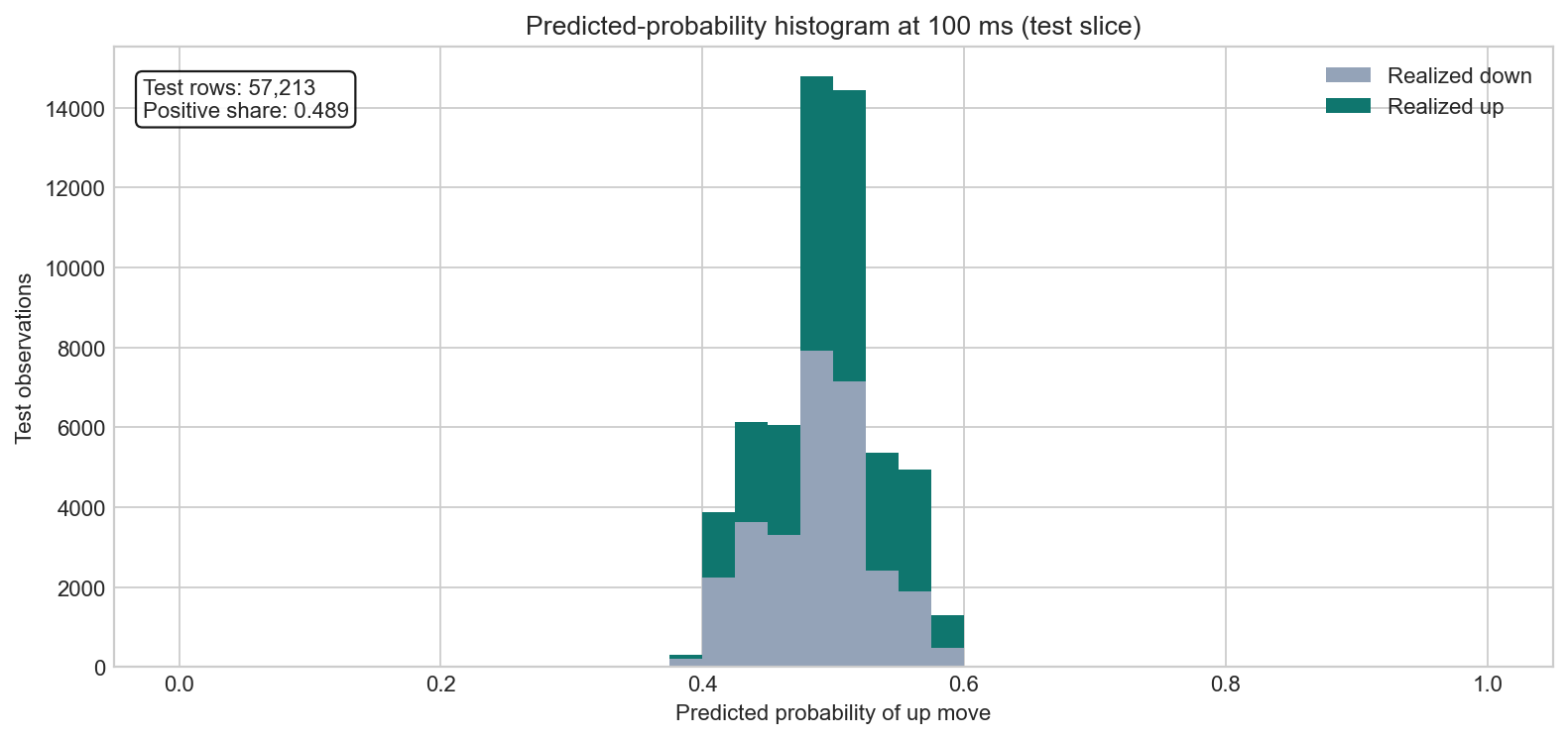
- Labels after sampling: 114,426 valid 1-second labels (49.4% positive, 50.6% negative); 95,902 no-change ties dropped (45.6% tie share). The high tie share reflects sub-tick-stable mid-prices in 2012 when the top-of-book often did not move within 1 s.
- Quality status:
pass.
Tick rule. The pipeline takes the explicit aggressor side from LOBSTER's direction field when present and falls back to a sign-from-price-change tick rule when not. On this sample the aggressor flag is present for every trade, so no tick-rule inference was needed.
3. Feature and Label Construction
Let $b_{\ell,t},a_{\ell,t}$ and $q^{b}_{\ell,t},q^{a}_{\ell,t}$ denote the level-$\ell$ bid/ask prices and visible sizes at event time $t$. Mid-price and spread are
The top-five depth imbalance is
The prior-one-second signed-trade imbalance, with $\tau_i$ the trade timestamp and $s_i\in\{-1,+1\}$ its aggressor sign, is
The cadence sampler chooses the most recent event-time state $\le$ each grid timestamp using a backward as-of merge with a 1 s tolerance, so no feature value uses information from after $t$. The forward label uses the first sampled mid at or after $t+h$ ($h=1$ s) and is recorded together with its source future timestamp for audit.
Worked example (real row, 100 ms cadence). At one sampled snapshot in the test window, the state has $b_1=583.06,\;a_1=583.19,\;\mathrm{spr}_t=13$ ticks, $\sum q^b_{1..5}\approx 2{,}010,\;\sum q^a_{1..5}\approx 1{,}730$, giving $I_t^{(5)}\approx 0.072$. The prior-second signed trade volume is negative against positive absolute, so $T_t^{(1\mathrm{s})}<0$. If the future mid one second later equals the current mid, the snapshot is a no-change tie and is dropped from the labeled panel; if it moves up by at least one tick, the snapshot enters the panel with $y=1$. In either case, the label construction remains leakage-safe because the future lookup is anchored strictly at or after $t+h$.
4. Model and Baselines
We fit logistic regression with $\ell_2$ regularization (regularization_strength $=10^{-4}$) on standardized features via L-BFGS-B, after replacing per-feature NaNs with the training-set median in the modeling pipeline. Three models are evaluated on the same chronological split:
- constant — predicts the training base rate;
- imbalance_only — $I^{(5)}_t$ as the sole regressor;
- full — $\{I^{(5)}_t,\,\mathrm{spr}_t,\,T^{(1\mathrm{s})}_t\}$.
| Feature | Std. coefficient | Interpretation |
|---|---|---|
trade_sign_imbalance_1s | $-0.154$ | Largest magnitude; negative sign $\Rightarrow$ short-horizon mean reversion. |
imbalance_top5 | $+0.077$ | Half the magnitude of trade-sign; heavier bid depth predicts up. |
spread_ticks | $+0.042$ | Small positive contribution; widest spreads weakly precede up moves. |
intercept | $-0.005$ | Effectively zero — training class share is 49.4% positive. |
What this says. On this real sample, trade-sign imbalance is the largest single contributor in the full model, and it points the opposite direction from a naive momentum reading. Recent aggressor buying is followed, on average, by a small reversal of the mid one second later — consistent with temporary price impact and partial liquidity replenishment. Depth imbalance contributes a smaller positive coefficient, and spread enters only marginally.
Feature-ablation (AUC & Brier on the test slice, 100 ms).
| Model | $n_{\mathrm{obs}}$ | AUC | Brier | Lift over constant |
|---|---|---|---|---|
| constant | 57,213 | $0.500$ | $0.2500$ | — |
| imbalance_only | 57,213 | $0.513$ | $0.2499$ | $+0.013$ |
| full | 57,213 | $0.567$ | $0.2467$ | $+0.067$ |
Depth imbalance alone clears $0.5$ but by less than two percentage points. The two added features — spread and trade-sign imbalance — raise AUC by another five percentage points. The trade-sign feature in particular does real, decoupled work; it is not redundant with depth imbalance.
5. Discrimination
6. Stratified Discrimination
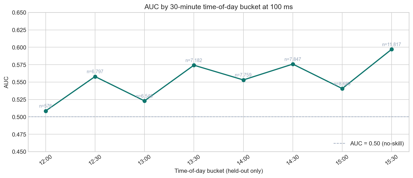
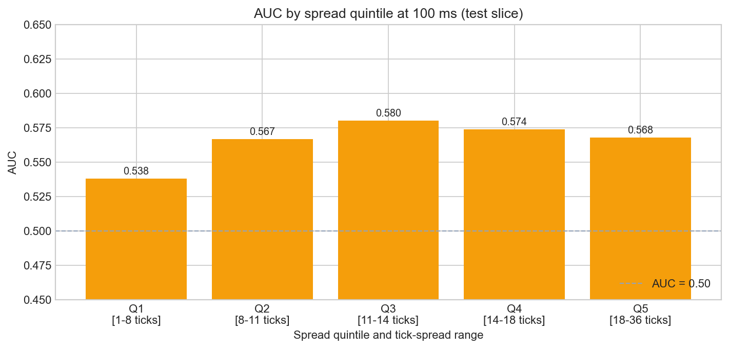
Where the signal lives. On this single-day sample, predictive discrimination is roughly U-shaped in spread regime and rises toward the close. The lift does not concentrate in the widest-spread quintile: Q3 dominates, while Q5 is unremarkable. The stratified result is therefore more nuanced than a simple “wider spreads imply stronger predictability” story.
7. Cadence Robustness
| Cadence (ms) | $n_{\mathrm{obs}}$ | $n_{\mathrm{pos}}$ | $n_{\mathrm{neg}}$ | AUC | Brier |
|---|---|---|---|---|---|
| 50 | 114,232 | 55,887 | 58,345 | $0.568$ | $0.2466$ |
| 100 | 57,213 | 27,995 | 29,218 | $0.567$ | $0.2467$ |
| 250 | 22,971 | 11,234 | 11,737 | $0.570$ | $0.2464$ |
Interpretation. AUC moves by less than $0.003$ across cadences and Brier by less than $0.0003$. This is a real robustness check on real data: at 50 ms many snapshots reuse the same event-book state because LOBSTER updates do not occur every 50 ms (backward-fill), while at 250 ms each snapshot reflects more information accumulated since the last sample. The signal is essentially scale-invariant on this day, which weakens the case for sub-100 ms snapshotting in production.
8. Cost-After-Execution
The decision rule converts probabilities into actions $d_t\in\{-1,0,+1\}$ via a symmetric threshold $p^\star$:
Per-action taker cost is $c_t = \mathrm{spr}_t \cdot \alpha + f \cdot m_t$ with full spread-crossing $\alpha=1$ and a 1 bp taker fee $f$. Net result is $r_t = d_t \cdot \Delta_h m_t - c_t \cdot \mathbf{1}\{d_t\ne 0\}$ and is scaled by a cost multiplier $\kappa\in\{0.5,1.0,1.5\}$ to stress-test the assumption.
| Threshold | Multiplier | $n_{\text{actions}}$ | No-trade share | Gross EV/obs | Net EV/obs | Net EV/action |
|---|---|---|---|---|---|---|
| 0.50 | 0.5 | 57,213 | 0.00 | 0.0041 | $-0.0895$ | $-0.0895$ |
| 0.50 | 1.0 | 57,213 | 0.00 | 0.0041 | $-0.1831$ | $-0.1831$ |
| 0.50 | 1.5 | 57,213 | 0.00 | 0.0041 | $-0.2768$ | $-0.2768$ |
| 0.55 | 0.5 | 16,584 | 0.71 | 0.0030 | $-0.0227$ | $-0.0782$ |
| 0.55 | 1.0 | 16,584 | 0.71 | 0.0030 | $-0.0483$ | $-0.1668$ |
| 0.55 | 1.5 | 16,584 | 0.71 | 0.0030 | $-0.0740$ | $-0.2553$ |
| 0.60 | 0.5 | 341 | 0.99 | 0.0001 | $-0.0003$ | $-0.0504$ |
| 0.60 | 1.0 | 341 | 0.99 | 0.0001 | $-0.0007$ | $-0.1188$ |
| 0.60 | 1.5 | 341 | 0.99 | 0.0001 | $-0.0011$ | $-0.1872$ |
negative_after_cost in every cell.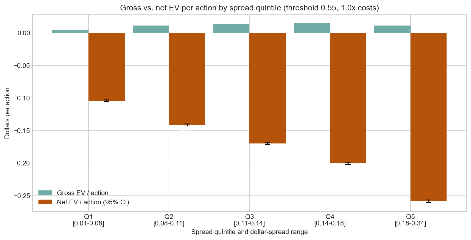
Spread vs. fee breakdown.
At the primary $0.55/1.0\times$ cell, the average per-action transaction cost is $\$0.177$. Decomposed:
- Mean spread cost: average test-slice spread $\approx 0.129$ dollars (12.9 ticks), full-spread crossing $\alpha=1$ $\Rightarrow$ $\$0.129$/action.
- Mean fee cost: 1 bp on $\overline{m_t}\approx\$582$ $\Rightarrow$ $\$0.058$/action.
Spread dominates fees by roughly $2.2\times$ on this instrument-day. The gross edge is $\sim\$0.003$/action; the model would need a $\sim 60\times$ improvement in per-action edge — or a maker-rebate execution model that recovers most of the spread — to clear cost.
Deployability. A simple deployability indicator can be written as
On this sample, the first two conditions hold (AUC clears chance, reliability tracks the diagonal); the third fails in every cell of Table 3. The indicator evaluates to $0$.
9. Discussion
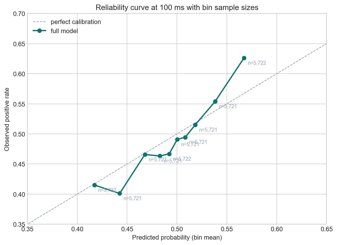
What the result says. On a real, full LOBSTER trading day for AAPL, the three-feature logistic specification picks up genuine one-second-ahead directional information: AUC of $0.567$, calibration close to the diagonal across the full $[0.42, 0.57]$ predicted-probability range, and a coefficient ranking that is robust under feature ablation. Most of the lift comes from prior-one-second trade-sign imbalance (with a negative sign — short-horizon mean reversion), not from depth imbalance, which contributes a smaller positive effect. The cadence ablation establishes that the result is not a sub-second artifact: the same AUC obtains at 50, 100, and 250 ms.
What the result does not say. The AUC does not survive a taker execution model. At every threshold and every cost multiplier in the sweep, net expected value is negative; the gross edge of $\sim\$0.003$/action sits well below the typical $\sim\$0.13$ spread on this instrument-day. This is the central cost-after-execution gap in the study. It also says nothing about persistence across days, instruments, or venues because the analysis is limited to one instrument-day. The widest-spread-quintile hypothesis is not borne out: Q3 (mid spreads) shows the highest AUC, and Q5 is unremarkable.
What would change the result. Three concrete moves would materially shift the conclusion. First, a maker-style execution model with partial-fill assumptions and a passive-rebate term would recover most of the spread; under any reasonable rebate this signal becomes a candidate for queue-jumping work rather than taker prediction. Second, queue-position features (own-order rank at top-of-book, plus arrival/cancellation rates at the inside) would let the signal condition on the local micro-state of the LOB rather than aggregate top-five depth. Third, a multi-day panel (LOBSTER samples exist for AMZN, GOOG, INTC, MSFT, SPY in addition to AAPL) would let us measure cross-day stability rather than report a point estimate that may be specific to 2012-06-21.
10. Limitations
- Single instrument. Results are reported for AAPL only; the LOBSTER event file is one ticker per release. No cross-sectional or cross-instrument variance estimate.
- Single day. 2012-06-21 is one trading day. This analysis does not measure cross-day stability and does not generalize.
- Single session segment for held-out evaluation. The chronological 70/30 split places 09:30–12:28 in training and 12:28–16:00 in test; we make no out-of-sample claim about the open. The early-test bucket (12:00) is the noisiest.
- High tie share (45.6%). The 1-second forward mid-price often does not change at all in 2012 AAPL; ties are dropped by construction of the binary up/down label, and the dropped share is large enough that the labeled panel is roughly half the snapshot count.
- Taker execution only. The cost overlay assumes full spread crossing on every action. No maker / queue-position model is included; the negative result is a taker result.
- No queue-position feature. Depth aggregates rather than own-order rank or LOB micro-events; queue-position features are the clearest next extension.
- No cross-venue replication. The Binance BTC/USDT path is not run here, so the evidence is limited to the LOBSTER AAPL sample.
- Trade-sign reliance on aggressor flag. On this LOBSTER sample 100% of trades carry an explicit aggressor; on samples or venues where the flag is missing, the tick-rule fallback would introduce additional noise into the dominant feature.
A. Full Coefficient Table (Appendix A)
| Model | Feature | Coefficient | Fit method |
|---|---|---|---|
| constant | intercept | $\phantom{-}0.499$ | constant_base_rate |
| imbalance_only | imbalance_top5 | $\phantom{-}0.042$ | logistic_regression_scipy |
| imbalance_only | intercept | $-0.005$ | logistic_regression_scipy |
| full | imbalance_top5 | $\phantom{-}0.077$ | logistic_regression_scipy |
| full | spread_ticks | $\phantom{-}0.042$ | logistic_regression_scipy |
| full | trade_sign_imbalance_1s | $-0.154$ | logistic_regression_scipy |
| full | intercept | $-0.005$ | logistic_regression_scipy |
B. Full Cost Cube (Appendix B)
| Cadence | Thr | Mult | $n_{\text{actions}}$ | Net EV/obs | Net EV/action | Status |
|---|---|---|---|---|---|---|
| 50 | 0.55 | 0.5 | 32,128 | $-0.0210$ | $-0.0747$ | neg. |
| 50 | 0.55 | 1.0 | 32,128 | $-0.0468$ | $-0.1664$ | neg. |
| 50 | 0.55 | 1.5 | 32,128 | $-0.0725$ | $-0.2580$ | neg. |
| 100 | 0.50 | 0.5 | 57,213 | $-0.0895$ | $-0.0895$ | neg. |
| 100 | 0.50 | 1.0 | 57,213 | $-0.1831$ | $-0.1831$ | neg. |
| 100 | 0.50 | 1.5 | 57,213 | $-0.2768$ | $-0.2768$ | neg. |
| 100 | 0.55 | 0.5 | 16,584 | $-0.0227$ | $-0.0782$ | neg. |
| 100 | 0.55 | 1.0 | 16,584 | $-0.0483$ | $-0.1668$ | neg. |
| 100 | 0.55 | 1.5 | 16,584 | $-0.0740$ | $-0.2553$ | neg. |
| 100 | 0.60 | 0.5 | 341 | $-0.0003$ | $-0.0504$ | neg. |
| 100 | 0.60 | 1.0 | 341 | $-0.0007$ | $-0.1188$ | neg. |
| 100 | 0.60 | 1.5 | 341 | $-0.0011$ | $-0.1872$ | neg. |
| 250 | 0.55 | 0.5 | 6,745 | $-0.0218$ | $-0.0750$ | neg. |
| 250 | 0.55 | 1.0 | 6,745 | $-0.0490$ | $-0.1668$ | neg. |
| 250 | 0.55 | 1.5 | 6,745 | $-0.0762$ | $-0.2585$ | neg. |
neg. $=$ negative_after_cost (every cell).C. Session Timeline (Appendix C)
References
- Cont, R. (2011). Statistical modeling of high-frequency financial data. IEEE Signal Processing Magazine.
- Cont, R., Kukanov, A., and Stoikov, S. (2014). The price impact of order book events. Journal of Financial Econometrics.
- Lipton, A., Pesavento, U., and Sotiropoulos, M. (2013). Trade arrival dynamics and quote imbalance in a limit order book. arXiv:1312.0514.
- Cartea, A., Jaimungal, S., and Penalva, J. (2015). Algorithmic and High-Frequency Trading. Cambridge University Press.
- Bouchaud, J.-P., Bonart, J., Donier, J., and Gould, M. (2018). Trades, Quotes and Prices: Financial Markets Under the Microscope. Cambridge University Press.
- Easley, D., López de Prado, M., and O'Hara, M. (2013). High-Frequency Trading: New Realities for Traders, Markets and Regulators. Risk Books.
- Huang, R. and Polak, T. LOBSTER: Limit order book reconstruction system. https://lobsterdata.com.
- Binance. Binance API Documentation: Order Book and Depth Streams. https://developers.binance.com/docs/binance-spot-api-docs/web-socket-streams.