Abstract

This report audits the reproducibility of Real-Time Machine Learning in the Cross-Section of Stock Returns (Li, Rossi, Yan & Zheng, Journal of Financial Economics, 2025). Rather than the paper's headline 18,113-signal universe—generated from WRDS/Compustat fundamentals and not reproducible from public data—the audit targets the paper's Table 7 Chen–Zimmermann sub-analysis (207 published anomalies from the Open Source Asset Pricing March 2022 release), for which the paper reports a boosted-tree (BRT) equal-weighted $10\!-\!1$ return of $5.18\%$/month and an annualized Sharpe of $3.68$. The deliverable is two things: a fully engineered, leak-audited real-time training pipeline—expanding-recursive annual windows, a frozen 15-point hyperparameter grid, decile portfolio construction, six-factor alphas, and a trading-cost overlay—built to be auditable end to end; and an honest account of what could and could not be run from public inputs. The OSAP-exact Table 7 reproduction is blocked at a single, identifiable seam: OSAP ships its signals keyed by a CRSP security identifier alone, and no public, commercial-clean table maps that identifier to a tradeable ticker, so the 207-signal panel cannot be priced without CRSP/WRDS. That seam is documented precisely rather than papered over with a fabricated number. A second, commercial-use-clean track—an SEC-identifier universe with EDGAR XBRL fundamentals and a licensed price feed—runs end to end and produces an equal-weighted BRT Sharpe of 1.25 ($t=3.30$) on a post-2009 large-cap universe. That spread survives six-factor risk adjustment (alphas of $1.2$–$1.5\%$/month, $t$ up to $4.6$), is not driven by short-term reversal, and is barely dented by trading costs—yet it collapses when the smallest names are removed or the legs are value-weighted, and a two-layer neural net and a linear model bracket it on either side. The report shows why this magnitude is economically meaningful yet not comparable to the paper's $3.68$, decomposes the runnable part of the gap, and draws governance lessons for any desk operating a similar real-time ML stack.

Scope honesty (read first). This audit replicates the paper's Table 7 / Chen–Zimmermann robustness check on published anomalies—not the paper's central Tables 1–2 claim that real-time ML on the full 18k-signal universe is weaker than the prior literature. That central claim requires the Yan–Zheng (2017) fundamental-signal construction (240 accounting variables $\times$ 76 transformations) from Compustat, which is not publicly reproducible. Every empirical number in this report carries Table 7 / CZ-sample scope and must never be read as a full-universe result.

Model governance is what separates a research firm from a backtesting shop. A careful, public replication audit of a recent, high-profile equity-ML paper is among the highest-leverage artifacts such a firm can publish: it signals methodological seriousness to allocators, demonstrates the ability to read and stress modern academic work rather than merely consume its conclusions, and produces a referenceable deliverable that later model-risk reviews can stand on.

Three design commitments make this audit a credential rather than a press release. First, the post-publication out-of-sample window is the product: allocators care less about whether an in-sample number matches to the basis point than about how a model held up after the anomalies it trades on were published, and because the target paper is itself about real-time implementability, that concern is native to the design—though, as §7 makes plain, the public-data track can honour it only in part. Second, honesty about scope is itself the credential: the paper's marquee result is not publicly reproducible, and even the robustness check that is reproducible runs into a hard data seam, so the credible move is to say so plainly, locate the seam exactly, and replicate only the part that genuinely can be, never mislabeling it as the headline. Third, a leak-free real-time protocol is non-negotiable: the methodological centerpiece is an expanding-recursive annual protocol in which the training set grows year by year and no future information can enter a forecast, with protocol-level look-ahead tests built into the pipeline rather than bolted on.

Li, Rossi, Yan & Zheng (henceforth LRYZ) ask whether ML return-prediction strategies are truly implementable in real time, or whether their reported performance benefits from hindsight about anomalies that were only published later. Their headline finding is sobering: on a universe of 18,113 fundamental signals built in the Yan–Zheng (2017) permutational style, a real-time boosted regression tree earns an equal-weighted $10\!-\!1$ spread of only $0.95\%$/month ($t=6.63$, Sharpe $1.02$) and a value-weighted spread of $0.40\%$/month ($t=2.34$, Sharpe $0.30$)—substantially weaker than the numbers the prior anomaly-ML literature had led readers to expect.

The paper anticipates the obvious objection—“maybe the ML is just bad”—with a battery of robustness samples. Table 1 maps the paper's structure and isolates the one cell this audit can faithfully target.

Exhibit	Content	Reproducible publicly?
Tables 1–2	Central claim. BRT decile portfolios over the full 18,113 fundamental signals; EW $10\!-\!1 = 0.95\%$/mo, VW $=0.40\%$/mo.	No — needs Compustat / Yan–Zheng construction.
Table 3	Large- vs. small-cap subsamples on the 18k universe.	No.
Table 4	Neural nets NN1–NN5; shallow beats deep.	Partially (shape check only).
Table 5	Past-return (Martin–Nagel) signal universe.	No.
Table 6	Green–Hand–Zhang (2017) 94-anomaly sample.	Partially.
Table 7	Chen–Zimmermann 207-anomaly sample (OSAP Mar. 2022). BRT EW $10\!-\!1 = 5.18\%$/mo, Sharpe $3.68$; VW $=2.32\%$/mo. The “ML matches prior literature on published anomalies” check.	Target of this audit.
Table 9	Short-term-reversal–excluded CZ robustness.	Secondary target (§7.4).
Table 11	Chen–Velikov net-of-cost returns on the 18k universe.	Overlay (CZ scope).

The annual frequency is essential and easy to get wrong: LRYZ predict annual July$(t)$ $\to\,$June$(t{+}1)$ excess returns, refit annually, hold for twelve months, and rebalance once a year (§2.2.1). Every design choice below assumes this annual cadence.

Replicating Table 7 demonstrates that an OSAP-plus-boosting-plus-public-price pipeline can reproduce prior-literature-magnitude alphas on published anomalies. It does not test the paper's central claim, because the 18k universe cannot be built from public data. The audit's value therefore lies in pipeline validation, a post-publication read on a public-data anomaly composite, and a gap decomposition that attributes the difference to identifiable sources.

In the course of the work the project split into two tracks, both engineered behind a single interface and schema layer. Track A—the OSAP headline (paper-faithful, academic)—targets Table 7 directly: the OSAP March 2022 207-signal library, a CRSP-substitute price panel, and the paper's exact protocol. It is fully engineered and tested, but its production headline run is blocked at the identifier seam: OSAP distributes its signals keyed by a CRSP security identifier and a year-month only, with no shipped ticker or CUSIP, and no public, commercial-clean table bridges that identifier to a tradeable ticker. Without that bridge the 207-signal panel cannot be priced from a public feed, so no OSAP Table-7 number is reported (§6). Track B—the commercial-clean public track (ticker-native)—removes all WRDS/CRSP/Compustat dependencies and their non-commercial academic licensing by using the SEC company-ticker universe with the central index key (CIK) as the entity id, SEC EDGAR XBRL fundamentals (point-in-time by filing date), and a licensed price feed. It recomputes a focused anomaly subset rather than the OSAP 207, runs end to end on real data, and is the source of every live result in §7.

The split is itself a governance finding: the identifier and licensing constraints on the canonical academic data are as binding as the statistical questions, and a deployable pipeline has to be designed around them from the start. The seam that blocks Track A—an identifier with no public route to a ticker—is the very thing Track B dissolves by choosing a public, ticker-mappable universe.

Series	Source / vintage	Role & caveat
Anomaly signals (A)	Open Source Asset Pricing, March 2022 release (Chen–Zimmermann; 207 anomalies)	Paper-exact pin (§3.6 fn. 19); keyed by a CRSP identifier only.
Universe (B)	SEC company-ticker list; entity id = CIK	Public, commercial-clean; the SEC publishes the CIK$\leftrightarrow$ticker map.
Fundamentals (B)	SEC EDGAR XBRL fundamentals, point-in-time by filing date	Public domain; the XBRL mandate means the panel begins $\sim$2009.
Prices / market cap	yfinance (A, CRSP substitute); Tiingo EOD (B, licensed feed)	Survivorship plus no delisting returns is the central data risk.
FF3, FF5, MOM, RF	Ken French data library	Standard; the Sharpe denominator uses the French risk-free rate.
Q-factor (ROE, IA, $\dots$)	Hou–Xue–Zhang	Q-factor alpha row; the panel ends Dec 2024.
Trading costs	Chen–Velikov (2022) LF effective spreads	Ends 2017; Track B (2019–25) uses a fixed-bp grid instead (§7.7).
Macro state	FRED recession and VIX series, Wurgler sentiment, Pastor–Stambaugh liquidity	Sub-period diagnostics (Track A scope).

The two price sources are a deliberate choice. Track A uses yfinance as a CRSP substitute—a deliberately weak proxy with no delisting returns and a survivorship-prone constituent list, instrumented with universe-coverage and delisting-sensitivity diagnostics. Track B uses a licensed feed because a commercial showcase cannot rest on non-commercial academic data, nor on free price-data tiers whose terms are likewise non-commercial. The pipeline is identical across price vendors: a new vendor is a single loader implementation, not a pipeline change.

The pipeline is a sequence of validated stages, each recording its row counts, source vintages, runtime, and warnings into a run manifest. The empirically load-bearing stages are described below.

Signals for formation year $t$ are paired with the forward annual excess return, following the Fama–French (1992) publication-availability convention. The target is the compounded July-to-June excess return,

so that signals dated $t$ never see returns that postdate their formation.

Each raw signal is mapped, within each cross-section, to a rank scaled to $[-1,+1]$, and missing values are imputed to $0$ (the cross-sectional median by construction)—the GKX and paper convention (§2.3, fns. 11–12). For $N_t$ non-missing observations of signal $s$ with cross-sectional rank $\rho_{i,t}\in\{1,\dots,N_t\}$,

Because only the ordering survives this transform, a level-vs-log choice for any single predictor is immaterial—a fact the audit exploits when proxying the identifier-gated signals (§6) and verifies directly with a missing-value ablation (§7.4).

This is the centerpiece. Let the panel start in year $y_0$, with an initial training span of $L$ years and a validation span of $V$ years. For each test year $\tau$ with $\tau \ge y_0 + L + V$, the window is

The paper uses $L=V=12$; Track B uses a shortened $L=6,V=4$ (justified in §7). Training expands recursively while validation rolls forward at fixed length, so the first forecast uses $L+V$ years of history and no window ever touches data on or after its test year. The implementation enforces $y_0 \le \text{train\_end} < \text{val\_start} \le \text{val\_end} < \tau$ as a hard invariant and runs two leak guards on every fit: one forbids any feature column from equalling the target to numerical tolerance, and the other forbids access to any year at or beyond the test year. A dedicated leak test is part of the suite.

The headline model is a boosted regression tree (LightGBM), selected over the paper's exact 15-point grid (§2.3 fn. 9):

For each window, every grid point is fit on train and scored on validation by MSE; the minimiser (ties broken by the smaller tree-count-times-learning-rate product, for determinism) is refit on train$\cup$validation and applied once to the test year. Per-window selections are content-hashed and cached so reruns are auditable and cheap. Two comparison models share the same protocol harness and are both run live on Track B (§7.4): a linear elastic-net-style OLS baseline, and a single two-layer $[32,16]$ NN2 shape-check, the neural net using its validation split for early stopping rather than the boosting grid search.

Within each test year, stocks are sorted into deciles on the model's prediction; the strategy is long decile 10, short decile 1, held for the twelve months July$(t)\to$June$(t{+}1)$, in both equal-weighted (EW) and value-weighted (VW, on formation-June market cap) form. For a monthly $10\!-\!1$ series $\{R_m\}$ the reported statistics are

with Newey–West HAC standard errors (6 lags), plus annualized mean, volatility, and maximum drawdown. Risk-adjusted alphas come from time-series regressions $R_m=\alpha+\beta'f_m+\varepsilon_m$ under six factor models—CAPM, FF3, Carhart, FF5, FF5+MOM, and the Hou–Xue–Zhang Q-factor model—again with NW(6) $t$-statistics (§7.3).

Net returns use Chen–Velikov (2022) low-frequency effective spreads (the paper's choice) where the data exist, through 2017. Because Track B's holding window is 2019–2025, entirely past the Chen–Velikov cutoff, its net-of-cost result instead uses a transparent fixed-bp sensitivity grid ($\{10,30,50\}$ bp per side) charged against measured annual turnover (§7.7). Low-frequency spreads are biased high versus modern high-frequency spreads (by 25–50 bp post-decimalization) but low versus total cost (no shorting or impact cost); both directions are flagged rather than choosing one.

Track A implements every stage above against the paper-pinned inputs and passes its unit, integration, and leak tests. The OSAP March 2022 release downloads in full—204 predictors from public OSAP, with three that route through WRDS in the standard access package reconstructed from public prices (Deviation D1 below)—and the boosting library fits cleanly on the machine. The blocker is neither of those. It is a single identifier seam.

OSAP distributes every signal as a panel keyed only by a CRSP security identifier and a year-month, with no shipped ticker or CUSIP and none in the March 2022 signal documentation. Forming portfolios requires a price and market-capitalization series for each identifier, but public price feeds are keyed by ticker, and no public, commercial-clean table bridges the CRSP identifier to a tradeable ticker. The canonical crosswalk is the CRSP security-name file behind WRDS, which is both access-gated and non-commercial; gray community crosswalks are licensing-ambiguous and survivorship-biased on exactly the delisted names that matter. The 207-signal panel therefore cannot be priced without CRSP/WRDS, and no OSAP Table-7 alpha is claimed in this report. Reporting a number from a partial or mis-linked panel would be a governance failure; locating and naming the seam is the finding.

Two smaller, honestly labelled choices sit underneath it. The three WRDS-routed predictors—price, size, and short-term reversal—are reconstructed from the public price panel as the June nominal close, June market equity, and June one-month return, and recorded as proxies in the run manifest; because every signal is rank-transformed, these level proxies are adequate as proxies and are auto-superseded if native OSAP columns ever arrive. They are not the blocker—they fill in cleanly—the identifier bridge is.

Even blocked, Track A yields a production compute profile, measured on dimension-matched synthetic data at full production scale (207 signals $\times$ 4,000 stocks/year $\times$ the $12+12$ protocol). The first window—48k training rows, 96k train-plus-validation rows, 15 fits—takes $117.6$ s; the full 11-window expanding sweep is about $1{,}557$ s ($\approx$25.9 min) of wall-clock, with a peak resident set of $428$ MB on 12 logical cores. Selected hyperparameters cluster at a $0.01$ learning rate with $750$–$1{,}000$ trees (Table 3). Boosting cost scales with rows $\times$ features $\times$ trees, all of which match production, so the timing is representative even though the feature values are synthetic—the moment an identifier bridge lands, the headline run is a roughly half-hour job, not a re-engineering effort.

Quantity	Value
Grid points per window	15
Forecast windows (full sweep)	11
First-window wall-clock	117.6 s
Full expanding-sweep wall-clock (est.)	1,556.8 s ($\approx$25.9 min)
Panel rows / signals / stocks-per-year	140,000 / 207 / 4,000
Peak resident memory	428.2 MB
Modal selected hyperparameters	lr $=0.01$, trees $\in\{750,1000\}$

Track B is the part of this study that ran on real data end to end. Its results are genuine and reproducible from the committed artifacts; they are also, by construction, not comparable in magnitude to the paper's CZ-sample headline, and the reasons are stated explicitly.

Track B is not the paper. Universe = SEC filers (CIK id), prices = a licensed feed, fundamentals = SEC XBRL (post-2009). It recomputes a 17-signal anomaly subset on a post-2009 large-cap universe under a shortened $6{+}4$ protocol. The universe, window, signal set, and protocol all differ from the OSAP CZ sample, so a Sharpe of $1.25$ here is not evidence about the paper's $3.68$.

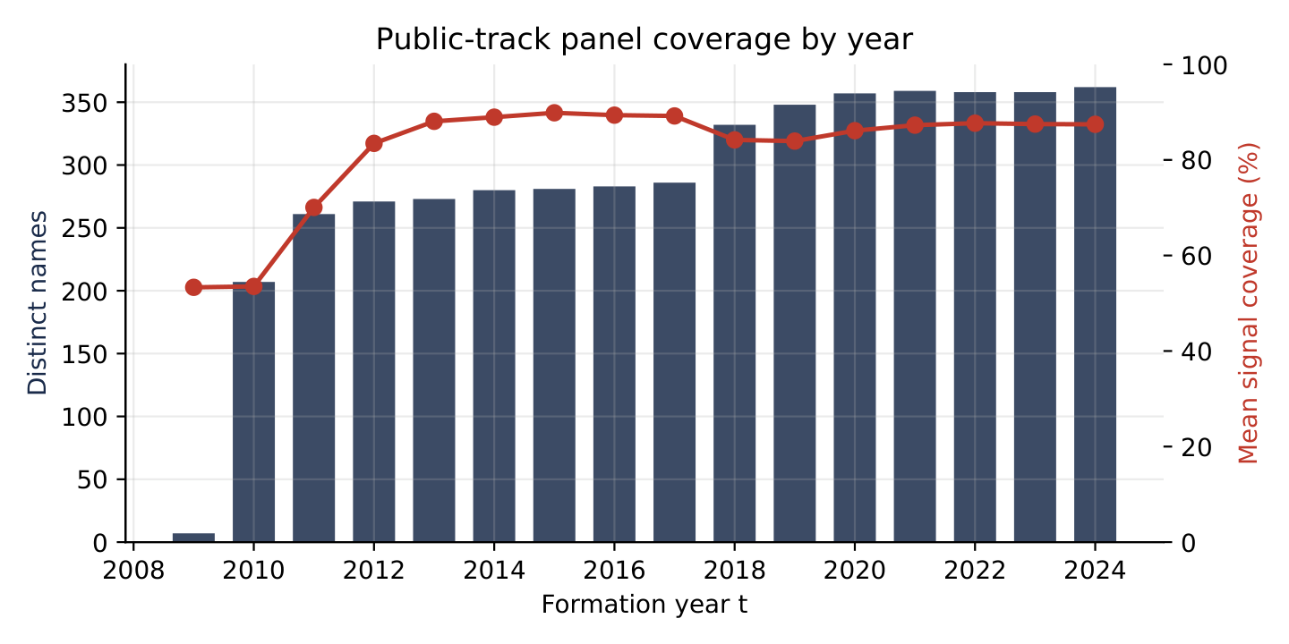
SEC XBRL begins at the $\sim$2009 mandate, so the fundamentals-bearing panel spans 2009–2024: 394 names, 4,623 firm-years ($\approx$289 names/year), 17 ranked signals, with overall signal coverage of 84.6%. Figure 1 shows coverage building as XBRL adoption matures and the universe fills in. Three consequences of this short, large-cap panel drive every downstream caveat. First, the protocol must be shortened: sixteen years cannot support the paper's $12+12$, which needs 24 years before the first forecast, so Track B uses $6+4$, making test year 2019 the first forecast and giving six forecast windows (2019–2024) and 72 holding months (July 2019–June 2025). Second, no in-sample-versus-post-publication decay comparison is possible: because the first forecast year (2019) is already after the paper's sample ends (June 2019), every Track B holding month is post-publication, there is no pre-publication in-sample leg on this panel to decay from, and the McLean–Pontiff-style decay measurement the motivation calls for cannot be formed here. That is a structural consequence of the XBRL start date, not an omission, and a per-forecast-year view (§7.6) stands in for it. Third, the universe is a free-tier, large-cap set: the price feed's free tier caps unique symbols, so the universe is the $\sim$470 largest SEC filers, and because anomaly returns concentrate in smaller stocks, value-weighting this large-cap set should—and does—dampen the spread sharply (§7.2, §7.4).

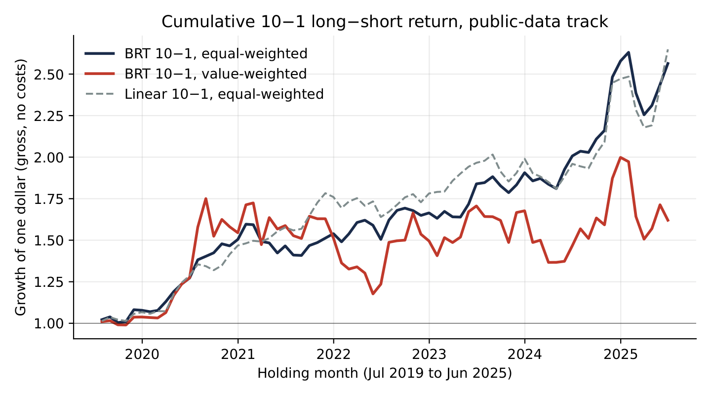
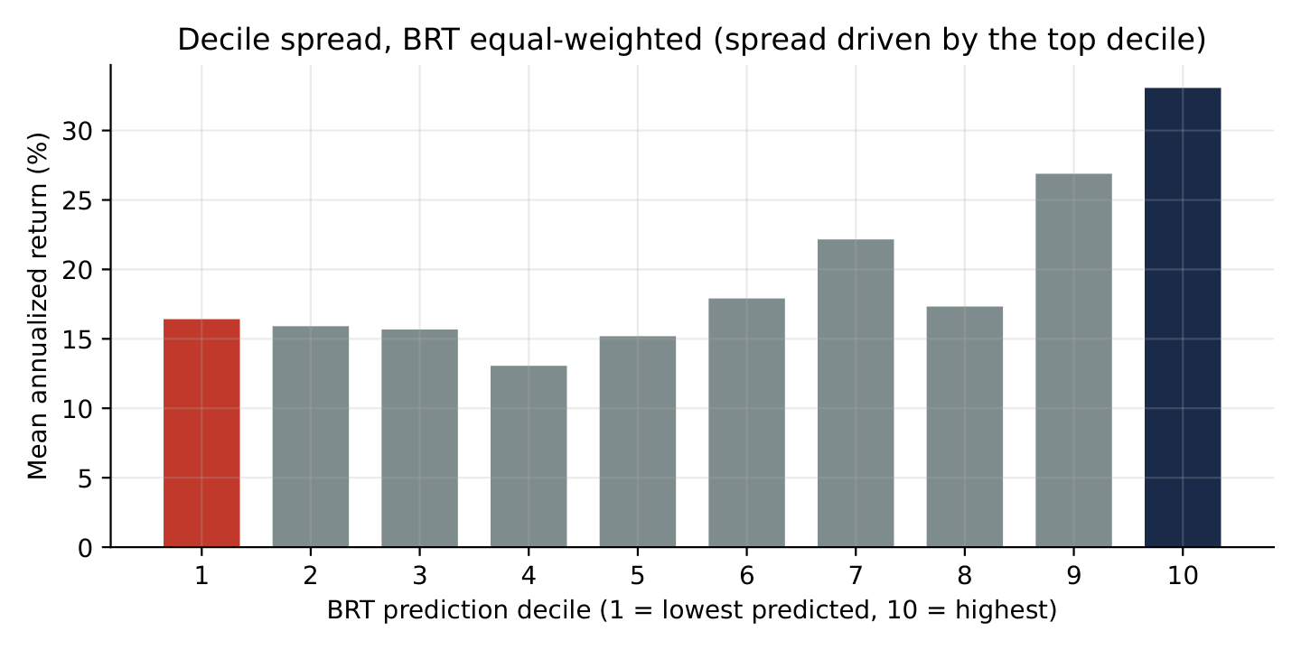
The boosted-tree $10\!-\!1$ portfolio earns an equal-weighted 16.6%/year ($1.387\%$/month) at an annualized Sharpe of 1.25 with a Newey–West $t$-statistic of 3.30; the value-weighted spread is $11.5\%$/year ($0.955\%$/month) at Sharpe $0.43$ ($t=1.20$)—statistically indistinguishable from zero (Table 4). The equal-weighted-over-value-weighted gap is exactly the smaller-cap concentration of anomaly returns operating on a large-cap universe, and the VW drawdown ($-33\%$ versus EW's $-14\%$) reflects the handful of mega-caps that dominate the value-weighted legs. Figure 2 plots the cumulative growth of one dollar in each leg, and Figure 3 shows the per-decile mean return. The spread is real but top-heavy: it is driven mainly by decile 10 against a relatively flat middle, rather than by a clean monotone staircase—useful texture for anyone tempted to read a single Sharpe number as a uniform signal.

Metric ($10\!-\!1$)	Equal-weighted	Value-weighted
Annualized Sharpe	1.253	0.433
Mean return, %/month	1.387	0.955
Mean return, %/year (ann.)	16.65	11.46
Annualized volatility, %	13.29	26.47
Newey–West $t$-stat (6 lags)	3.30	1.20
Maximum drawdown, %	$-14.3$	$-32.8$
Mean round-trip turnover, %/yr	134	134
Net Sharpe @ 50 bp/side	1.216	0.414
Months	72	72

The equal-weighted spread is not a factor exposure in disguise. Across all six factor models the EW $10\!-\!1$ alpha is $1.2$–$1.5\%$/month with Newey–West $t$-statistics between $2.9$ and $4.6$; the Carhart and FF5+MOM alphas ($1.28$ and $1.34\%$/mo, $t>4$) confirm that momentum does not absorb it, and the Q-factor alpha ($1.48\%$/mo, $t=3.5$) survives the investment and profitability factors (Table 5). The value-weighted alphas, by contrast, are economically smaller and statistically insignificant ($t\le1.9$ in every model)—the same equal-over-value story the raw spread tells, now visible through a risk-model lens.

	CAPM	FF3	Carhart	FF5	FF5+MOM	Q-factor
EW $\alpha$	1.16	1.40	1.28	1.47	1.34	1.48
($t$)	(2.85)	(4.22)	(4.08)	(4.61)	(4.49)	(3.47)
VW $\alpha$	0.48	0.85	0.62	0.89	0.58	1.21
($t$)	(0.65)	(1.72)	(1.34)	(1.76)	(1.23)	(1.90)

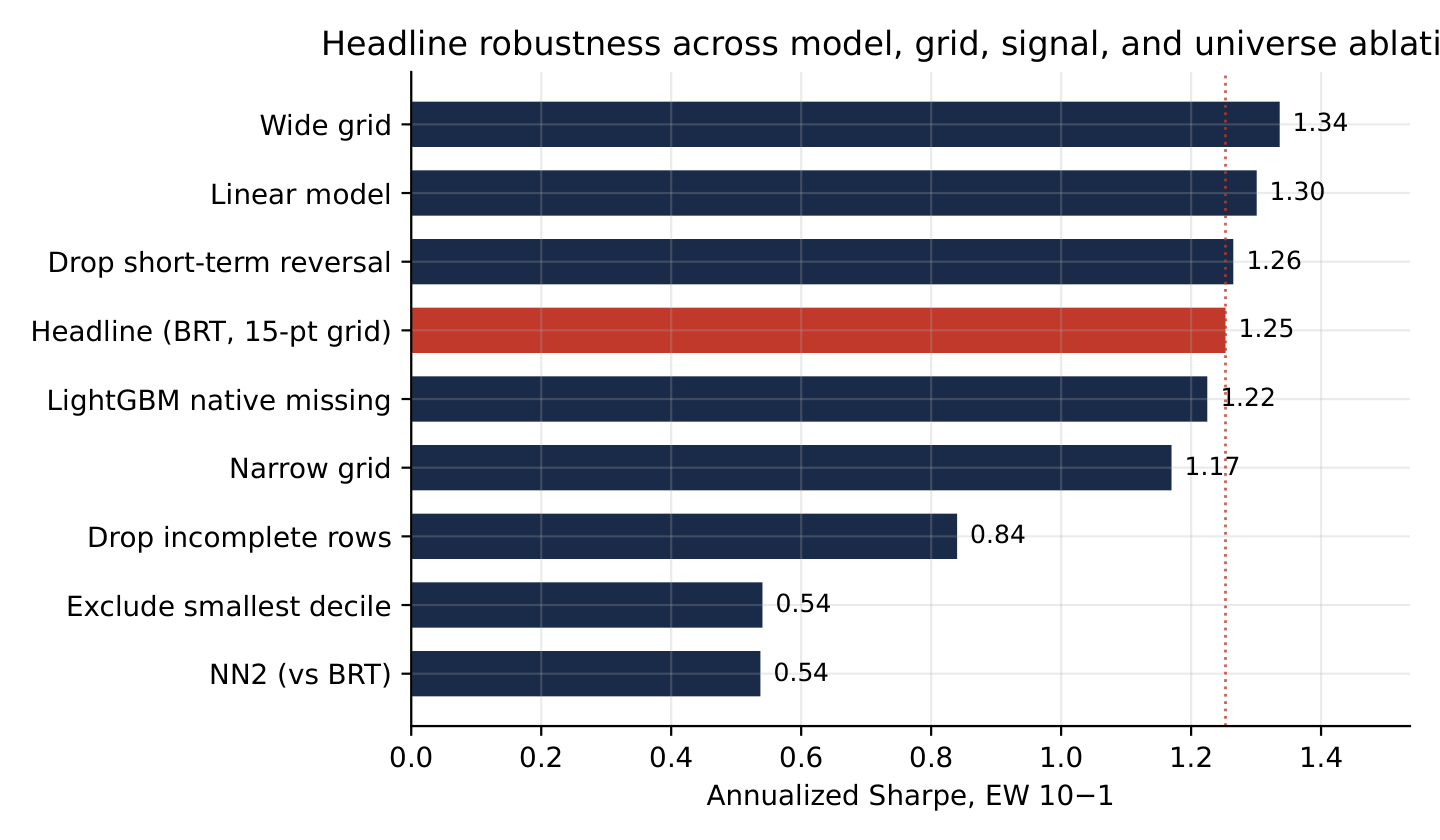
The headline survives—or fails in interpretable ways—across the ablations the panel permits (Table 6, Figure 4), and four findings stand out. The spread is not a short-term-reversal artifact: dropping the one-month reversal signal leaves the EW Sharpe essentially unchanged ($1.265$ versus $1.253$) and actually raises the VW Sharpe ($0.76$ versus $0.43$), echoing the paper's similarly modest CZ STR-excluded result ($5.18\!\to\!4.87\%$/mo). Size concentration is the dominant lever: removing the smallest within-panel size decile cuts the EW Sharpe by more than half, to $0.54$, and value-weighting cuts it to $0.43$—both point at the same mechanism, the premium living in the smaller names, and both are consistent with the anomaly literature and the paper's own size cautions. Complexity is not rewarded: a two-layer NN2 underperforms the boosted tree badly (EW Sharpe $0.54$ versus $1.25$) while a plain linear model slightly beats it ($1.30$), because on a 17-signal, $\sim$289-name annual panel there is little non-linear structure to exploit—an echo of the paper's “shallow beats deep” motif and a reminder that complexity must be earned. And imputation is not load-bearing: letting the booster handle missing values natively reproduces the headline ($1.225$), confirming the paper's remark that performance is similar without median-imputation, while dropping every row with any missing signal is degenerate here—only $7.6\%$ of firm-years are fully observed, so the panel thins by a forecast window and the Sharpe falls to $0.84$, which is itself the finding that the accounting signals are sparse early and zero-imputation is doing real work. Widening or narrowing the hyperparameter grid moves the EW Sharpe by only $\pm0.08$, and the long-window ablations remain skipped because the post-2009 panel cannot form windows that need 22–30 years before the first forecast—reported as skipped rather than silently omitted.

Ablation	Model	Status	Sharpe EW	Sharpe VW	$\Delta$ EW	Paper ref.
headline	BRT	completed	1.253	0.433	$0.000$	Table 7
grid_narrow	BRT	completed	1.170	0.547	$-0.083$	§2.3 fn. 9
grid_wide	BRT	completed	1.336	0.557	$+0.083$	§2.3 fn. 9
exclude_strev	BRT	completed	1.265	0.760	$+0.012$	Table 9
missing_native	BRT	completed	1.225	0.791	$-0.028$	§2.3 fn. 12
missing_drop_row	BRT	completed$^\dagger$	0.840	0.729	$-0.413$	§2.3 fn. 12
model_linear	linear	completed	1.301	0.840	$+0.048$	Table 4 analog
model_nn2	NN2	completed	0.537	0.428	$-0.716$	Table 4 analog
exclude_microcap	BRT	completed$^\ddagger$	0.540	0.538	$-0.713$	Table 3 analog
window_10_12 $\dots$ 18_12	BRT	skipped	—	—	—	Table IA.2

$^\dagger$ Degenerate: only $7.6\%$ of firm-years are fully observed, so the panel thins to 5 forecast windows. $^\ddagger$ Drops the smallest within-panel decile; the large-cap universe contains no true NYSE microcaps.

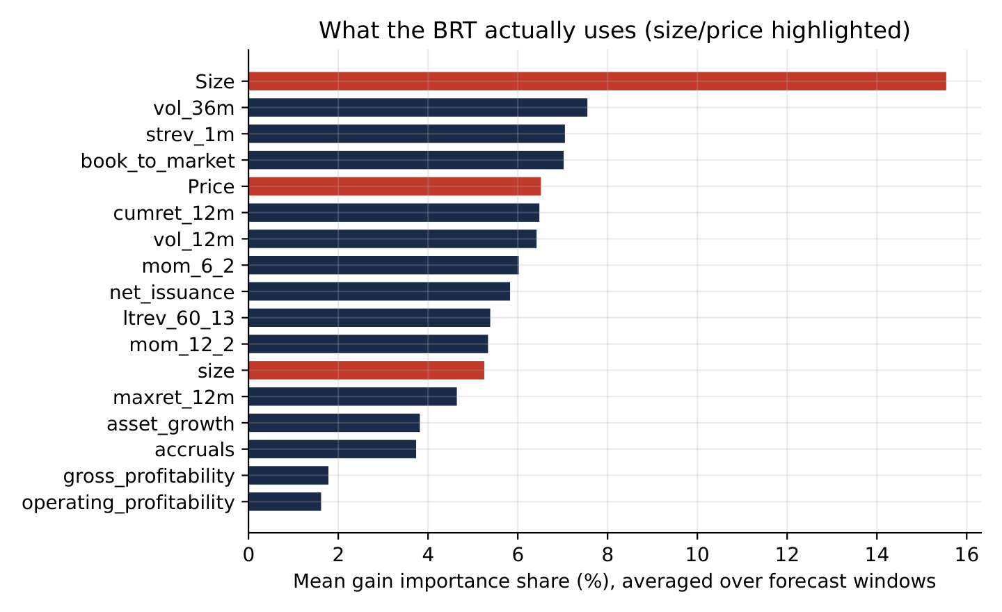
A governance audit should be able to say which signals a model leans on, not just how it scores. Figure 5 reports BRT gain importance averaged over the six forecast windows, and the picture is coherent with the ablations: size and price characteristics dominate. The size proxy alone is $15.5\%$ of total gain, and together the two size measures plus the price level account for roughly $28\%$; volatility, reversal, value, and momentum signals form a broad middle band; and the sparsely-populated accounting fundamentals (gross and operating profitability) sit at the bottom. This is exactly why removing the smallest size decile (§7.4) guts the spread: the model's single most important axis is size, and the premium it captures lives in the smaller names. It also flags a redundancy—the panel carries both a market-equity size proxy and an accounting size signal (Appendix B)—which a production build would collapse to one.

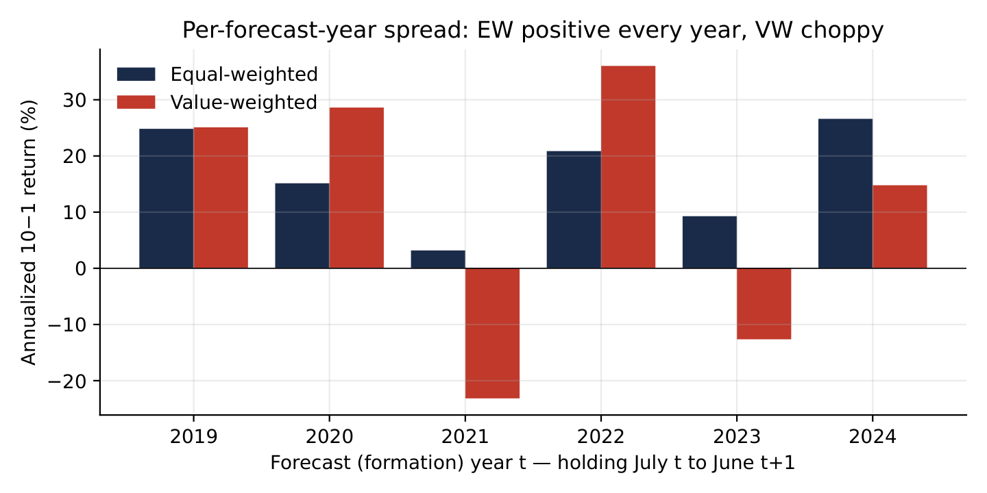
With no in-sample leg to decay from (§7), the honest substitute is to ask whether the composite has weakened across the six post-publication forecast years. It has not: the equal-weighted $10\!-\!1$ spread is positive in every year from 2019 to 2024 ($+25\%$, $+15\%$, $+3\%$, $+21\%$, $+9\%$, $+27\%$), with no monotone fade (Figure 6). The value-weighted leg is far choppier—two negative years (2021 and 2023)—which is the year-by-year shadow of its weak full-sample Sharpe. The equal-weighted composite is durable over this window; it is simply small-cap-tilted.

Because the holding window (2019–2025) lies entirely past the Chen–Velikov 2017 cutoff, the paper-faithful low-frequency-spread overlay cannot be applied to Track B, and a fixed-bp sensitivity is reported instead. Measured annual one-way turnover averages $\approx67\%$ per leg ($\approx134\%$ round-trip), so even at an aggressive $50$ bp/side the equal-weighted net Sharpe is $1.216$ (gross $1.253$) and the net return is $16.1\%$/yr (gross $16.6\%$)—a trivial drag, because the strategy rebalances once a year. Costs are not what separates this composite from the paper's; the universe, breadth, and weighting are (§8).

The paper's CZ-sample BRT posts an EW Sharpe of $3.68$; Track B posts $1.25$. This gap is expected and attributable to design differences, not to a contradiction of the paper. Some of those differences can be run as counterfactuals on the public panel; the rest are structural and un-runnable from public data. Table 7 separates the two. The runnable levers are large and all point the same way: value-weighting ($-0.82$ Sharpe) and removing the smallest names ($-0.71$) each roughly halve the spread, confirming that the bulk of the magnitude difference is a size-and-weighting story, not an ML story. The residual to $3.68$ is then carried by the levers that cannot be reproduced—the OSAP 207-signal breadth versus the 17 here, the full CRSP cross-section versus $\sim$470 large caps, the $12{+}12$ window versus $6{+}4$, and the 1987–2019 sample versus a six-year post-publication window.

Lever	Mechanism	$\Delta$ Sharpe
Runnable on the public panel (measured)
Headline BRT EW	17 signals, $\sim$289 names, $6{+}4$, all-cap, EW	(1.253)
Drop short-term reversal	Table 9 robustness; premium is not reversal	$+0.01$
Linear instead of BRT	little non-linearity to exploit	$+0.05$
NN2 instead of BRT	complexity unrewarded on a thin panel	$-0.72$
Exclude smallest decile	premium concentrates in smaller names	$-0.71$
Value-weight (large-cap)	mega-caps dominate; small-cap premium muted	$-0.82$
Structural — not reproducible from public data
Signal breadth	17 recomputed vs. the curated CZ 207	($\downarrow\downarrow$)
Universe	$\sim$470 large caps vs. full CRSP cross-section	($\downarrow\downarrow$)
Protocol & sample	$6{+}4$, 2019–24 vs. $12{+}12$, 1987–2019	($\downarrow$)
Data quality	yfinance/Tiingo vs. CRSP (no delisting returns)	(ambiguous)

The disciplined reading is that a fully public, commercial-clean anomaly-ML pipeline produces an economically meaningful, statistically significant equal-weighted spread ($t=3.30$; six-factor alpha $t$ up to $4.6$) out of sample, while value-weighting it on a large-cap universe removes most of the premium—directionally consistent with both the anomaly literature and the target paper's caution about real-time implementability.

The audit is engineered so that any number traces to a configuration, a code path, and a data vintage. Thirteen frozen project decisions—scope tier, window, protocol, OSAP pin, grid, factor roster, cost model, imputation, filters, seeds, and acceptance bands—together with two labelled deviations are recorded in the decision log (Appendix A) and mirrored into versioned configuration, so changing one requires an explicit log update. Every live number in §7 is rebuilt from the committed processed panel and the central seed by the project's own modules—the committed ablation suite, an extended-results stage, and the figure generator—and the reconstructed equal- and value-weighted Sharpes ($1.253/0.433$) match the committed metrics to four decimals. The public-track run manifest records the effective configuration hash, per-stage row counts, runtime, and warnings, and pins the OSAP March 2022 vintage, the Chen–Velikov 2017 cost vintage, the single date-stamped seed, the public-track configuration, and the commit at which the panel was built; numpy, the booster, and the neural-net library all read that one seed, and no stage sets an ad-hoc seed.

A fail-closed production-validation gate refuses to pass on smoke or fixture paths, missing artifacts, placeholder report text, bad snapshot hashes, or a forbidden full-universe scope tag. Its required-artifact list is wired to the Track A OSAP headline, so it gates the blocked paper-faithful deliverable rather than this Track B note, whose governance evidence is the manifest, the deterministic reconstruction just described, and the test suite. Finally, the three identifier-gated OSAP signals and the entire commercial-clean track are recorded as labelled deviations with rationale and auto-superseding behaviour, never as silent substitutions.

Several limitations bound these claims. Nothing here speaks to the paper's central full-universe claim, which requires the Compustat and Yan–Zheng construction; the scope is Table 7 only. No OSAP Table-7 number is reported, because Track A is blocked at the identifier-to-ticker bridge; only its compute profile is. No decay measurement is possible on Track B, whose XBRL-era panel forecasts 2019–2024, all post-publication, with no in-sample leg to decay from—hence the per-forecast-year substitute. Track B magnitudes are not paper-comparable, for the reasons enumerated in §8. The microcap ablation is within-panel: the large-cap universe has no true NYSE microcaps, so excluding “microcaps” removes only the smallest large caps, which is suggestive rather than a clean Avramov-style test. The neural-net result is a single two-layer shape check, not the paper's NN1–NN5; it underperforms here, but that is a one-architecture result, not a neural-network verdict. The public price feeds are weak CRSP substitutes, with no delisting returns, no Compustat-listing filter, and survivorship in the constituent list that diagnostics make visible but cannot remove. Costs on Track B are fixed-bp rather than the Chen–Velikov panel, which ends in 2017 before the holding window. And earnings-day sensitivity is not run, because per-name earnings dates are unavailable from public sources; that slot is marked missing rather than faked.

Several lessons generalize to any desk running a similar stack. The first is to audit identifiers before models: the one thing that blocked the paper-faithful track was not compute or signal licensing but that OSAP ships a CRSP identifier with no public ticker bridge, so a security master should be mapped to a tradeable, commercially-clean identifier before a data vendor is chosen. The second is to make the real-time protocol a tested invariant, because look-ahead leakage is the single failure that invalidates an entire backtest—encode the window boundaries and leak guards as assertions with their own tests. The third is to report “skipped” and “degenerate” loudly: window ablations the data cannot support, and a drop-row policy that thins the panel to $7.6\%$, are first-class results, and the discipline that records a skip is what keeps a blocked headline from being quietly fabricated. The fourth is to look at what a model uses, not just its Sharpe—here, gain importance (size dominates) predicted the microcap-exclusion collapse before it was run, and importance and ablations should corroborate each other or the strategy is not understood. The fifth is to prefer the simplest model that clears the bar, since a linear model matched the boosted tree and a neural net underperformed both; complexity should be earned by out-of-sample lift, not assumed. The last is to run the audit as a series: the framework is a reusable template, and a second replication every six months compounds reputational credit far faster than one-off pieces.

This audit set out to test the reproducibility of a prominent real-time equity-ML paper, and the honest finding has three parts. Methodologically, a faithful, leak-audited real-time pipeline—expanding-recursive windows, the paper's exact grid, decile portfolios, six-factor alphas, and a cost overlay—can be built and verified end to end, and the paper-faithful OSAP track is ready to run the moment an identifier-to-ticker bridge is available. On scope, the marquee result is not publicly reproducible, and even the Table-7 robustness check is blocked at a single, nameable identifier seam, which this report locates rather than papers over. Empirically, the one configuration that runs fully on public, commercial-clean data delivers an equal-weighted boosted-tree Sharpe of $1.25$ ($t=3.30$) that survives six-factor adjustment and short-term-reversal removal, yet collapses under value-weighting and microcap exclusion and is bracketed by a linear model and a neural net—real, significant, well-understood, and yet correctly not comparable to the paper's $3.68$, for reasons enumerated rather than hidden. That gap between what the pipeline can prove and what the public data will allow is precisely the kind of finding a governance function exists to surface.

ID	Decision	Rationale (paper ref.)
0.1	Scope tier = Table 7 / CZ 207, not Table 1 18k	Only Table 7 is publicly reproducible (§3.6, Table 7).
0.2	Universe window 1990-07 – 2025-06	Public price coverage pre-1990 too sparse; 2020+ is the OOS extension.
0.3	Annual July–June target; expanding $12{+}12{+}1$	Paper's signals are annual; real-time recursive protocol (§2.2.1, 2.3).
0.4	OSAP March 2022 pin (207 signals)	Vintage of the paper's CZ sample (§3.6 fn. 19).
0.5	Boosted tree; single NN2 $[32,16]$ shape check	Practical BRT; bounded NN sanity check (§2.3, Table 4).
0.6	Report EW & VW; headline = EW BRT $10\!-\!1$ Sharpe	Paper reports both; EW is the strong reference (Table 7).
0.7	15-point grid $\{100..1000\}\times\{0.01,0.05,0.10\}$	Paper's exact grid (§2.3 fn. 9).
0.8	Alphas: CAPM, FF3, Carhart, FF5, FF5+MOM, Q	Paper-faithful roster; NW $t$-stats (§2.3).
0.9	Chen–Velikov LF spreads to 2017 + 10/30/50bp grid	Paper-faithful costs with a transparent truncation (§3.8).
0.10	Rank to $[-1,1]$ within year; impute missing $=0$	Median after rank scaling; GKX convention (§2.3 fns. 11–12).
0.11	Common-stock, ex-financials, price $\ge\$1$; Compustat filter not enforceable	First three approximable publicly (§2.1).
0.12	Centralized date-stamped seed across libraries	Reruns must be auditable (§2.3).
0.13	Acceptance bands: EW $\pm$30pp, VW $\pm$40pp, Sharpe $\pm$1.0, $t\ge3$	Public substitutes preclude exact equality (Table 7).
D1	Proxy the 3 identifier-gated OSAP signals from public prices	Rank-only transform makes level proxies adequate; auto-superseded by WRDS.
D2	Commercial-clean ticker-native (SEC CIK) track	CRSP/Compustat are non-commercial/academic; CIK is public and ticker-mappable.

The price- and volume-based signals (monthly) are six- and twelve-month momentum, twelve-month cumulative return, one-month reversal, long-term (months 13–60) reversal, the twelve-month maximum daily return, and twelve- and thirty-six-month volatility. The accounting signals from SEC XBRL are gross and operating profitability, accruals, asset growth, net issuance, book-to-market, and size. Two market-linked proxies—the price level and a market-equity size proxy—complete the set. The accounting size signal and the market-equity size proxy both encode firm size and are partly collinear; together with the price level they carry about $28\%$ of BRT gain (§7.5), so a production build would collapse them to a single size axis, while they are kept distinct here to mirror the OSAP acronym set the proxies stand in for. Every signal module emits a common annual long-format record—identifier, formation year, signal name, signal value—so the panel-building, preprocessing, and ablation stages consume them unchanged across both tracks (on Track B the identifier column carries the CIK).

The end-to-end headline path is a single ordered command sequence, and each stage validates its output against the shared schema layer and appends to the run manifest: download-osap $\to$ build-universe $\to$ download-prices $\to$ download-factors / -q-factor / -chen-velikov / -sentiment / -liquidity / -macro $\to$ reconcile-permno-ticker $\to$ build-panel $\to$ preprocess $\to$ train-brt ( /-linear /-nn ) $\to$ form-portfolios $\to$ evaluate $\to$ run-ablations $\to$ decompose-gap $\to$ render-figures $\to$ render-report $\to$ validate-production-run. The commercial-clean track substitutes a public-track assembly step (SEC universe, licensed prices, EDGAR fundamentals) ahead of panel building; a separate extended-results stage produces the NN2, signal, universe, missing-value, alpha, turnover, cost, importance, and per-forecast-year deliverables that the in-panel ablation suite does not emit.

The live results in §7 are reconstructed deterministically from the committed ablation-suite artifacts and the extended-results stage via the project's own analysis modules; the reconstructed equal- and value-weighted Sharpes ($1.253/0.433$ for the boosted tree, $1.301/0.840$ for the linear model) reproduce the committed metrics to four decimals. The figures are generated from the same reconstructed series. The public-track run manifest pins the OSAP March 2022 vintage, the Chen–Velikov 2017 cost vintage, the date-stamped seed, the public-track configuration, and the panel-build commit.