Abstract

On a matched U.S. regular-hours panel of 21 trading days the average share of intraday variance that SPY and BTC carry below five minutes differs by $+0.16$ percentage points (BTC minus SPY), with a 95% date-block bootstrap interval of $[-0.76, +0.90]$. That cross-asset gap is small, it does not survive a Kolmogorov–Smirnov test of distributional equality, and its sign flips under two of three wavelet boundary modes and under a 24-hour rather than matched-hours BTC panel. The more durable finding is methodological: the short-time Fourier transform and the discrete wavelet transform define the 60+ minute band so differently — one as a residual, the other as a low-pass approximation — that they disagree at the 5–32 percentage-point level on identical inputs and their daily band-share series are negatively correlated in three of four SPY bands and two of four BTC bands. Under this lens the cross-asset spectral signature inherits the decomposition more than the data. The headline cross-asset gap is therefore reported alongside its specification sensitivity, and the cross-method audit is the report's central contribution.

Under the primary 30-minute short-time Fourier transform with Hann taper and 50% overlap on 1-minute log returns aligned to U.S. regular trading hours,

on $n = 21$ paired trading days (date-block bootstrap, block length 5, $B = 2000$). The cross-asset two-sample Kolmogorov–Smirnov distance for the same band is $D = 0.19$ with $p = 0.85$ uncorrected ($p_{\text{Bonf}} = 1.0$). The central estimate is roughly $1\,\%$ of the SPY 1–5 minute base share, the bootstrap distribution crosses zero on $45.9\,\%$ of resamples, and the KS test cannot reject equality of the SPY and BTC daily distributions. The original framing of this project paired the cross-asset gap with the share of stress weeks on which the sign of the gap inverts; with only one stress week in the sample window that share is undefined and is reported as such rather than imputed.

The motivating question is whether equities and crypto, often described as interchangeable risk assets, carry distinguishable intraday spectral signatures, and whether any such signature is stable when conditioned on stress weeks. The exercise is also a calibration step for later work in the Deep Wave Research portfolio: every downstream filter, denoiser, or regime-detection routine that operates on these series implicitly assumes a frequency profile, so measuring that profile end to end is the right preliminary step.

This report makes three contributions.

1. A reproducible pipeline that ingests SPY 1-minute bars from yfinance, BTC/USDT 1-minute bars from the Binance public REST endpoint, and VIX daily closes from FRED, and produces a complete artifact set — primary band-share tables, sensitivity sweeps, stress labels, Kolmogorov–Smirnov results, bootstrap distributions, and a cross-method audit — pinned by a SHA-256 manifest.
2. A defensible cross-asset headline that is honest about its sample size. The available Yahoo intraday window for SPY is approximately 30 calendar days, so point estimates are reported with date-block bootstrap confidence intervals and the report avoids framing them as method-invariant facts.
3. A negative methodological finding worth its own attention: the short-time Fourier transform residual and the discrete wavelet transform approximation define the 60+ minute band so differently that the BTC-minus-SPY mean gap flips sign across decompositions even before any data subset is considered. This finding is promoted to the centre of the report rather than relegated to a robustness aside.

The raw inputs are pinned by SHA-256 in the run manifest. The SPY 1-minute OHLCV snapshot covers the rolling window that yfinance currently exposes; a live availability probe showed that any request older than roughly 30 calendar days is rejected with the explicit message “The requested range must be within the last 30 days,” so the deliverable is scoped to that window with a paid intraday vendor (Polygon, Alpaca, or IBKR) queued as a follow-up for a longer panel. The BTC/USDT 1-minute klines are pulled over a UTC-day-aligned window enclosing the SPY range, so the 24-hour BTC panel used in the robustness section covers complete calendar days. The VIX daily closes are used only for stress-week labelling.

Returns are computed as $r_{i,t} = \log P_{i,t} - \log P_{i,t-1}$ on a matched-session panel keyed to America/New_York regular trading hours (09:30–16:00 local), then converted to UTC for storage. This anchors the trading window in local time and avoids the daylight-savings drift that a literal “13:30–20:00 UTC” window would introduce. Sessions with greater than 5% missingness on either asset are dropped; on the published run no sessions were dropped from either asset.

The matched-session panel contains 21 RTH trading days. ISO-week labels yield 1 stress week (ISO week 21 of 2026: weekly BTC realized volatility crossed its 80th percentile), producing 2 stress sessions per asset and 19 calm sessions per asset. All distributional claims in this report are read against that sample size.

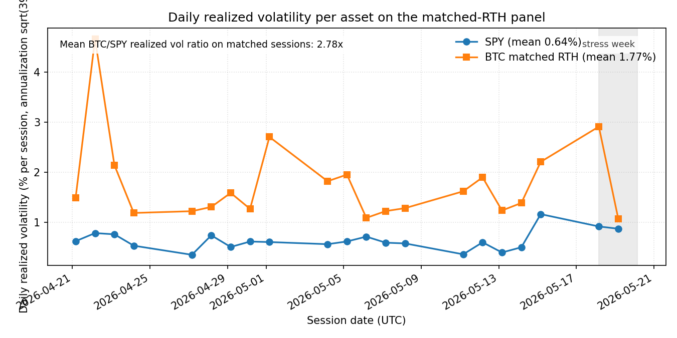
Spectral band shares are scale-free by construction. Before discussing them it is useful to anchor the comparison in absolute volatility, since a reader's natural prior is that BTC is simply more volatile than SPY rather than spectrally distinct from it. Figure 1 shows daily realized volatility per asset over the 21-day window, computed as the within-session standard deviation of 1-minute log returns annualized by $\sqrt{390}$. On the matched-RTH window BTC's realized vol is $2.78\times$ SPY's on average, with a single 4.7% session outlier on 2026-04-22 that is left in the panel. Whatever shape difference appears in the band-share comparison is therefore on top of an unambiguous absolute-volatility difference.

For each asset and each 1-minute return series the short-time Fourier transform with sampling frequency $f_s = 1/60~\mathrm{Hz}$ is computed as

with a Hann taper $w_n$, window length $N = 30$ minutes, and hop $h = N(1 - \rho) = 15$ minutes ($\rho = 0.5$). The four bands map to FFT bins by period $T = 1/\omega$:

• $1$–$5$ min: bins with $T \in [2, 5]$ minutes,
• $5$–$15$ min: bins with $T \in (5, 15]$ minutes,
• $15$–$60$ min: the 30-minute proxy bin (a single 30-minute window cannot resolve periods longer than $N$),
• $60+$ min: defined as a residual, $\mathrm{Var}_d - \sum_b P_b$ on each session $d$, where $\mathrm{Var}_d$ is the total within-session variance.

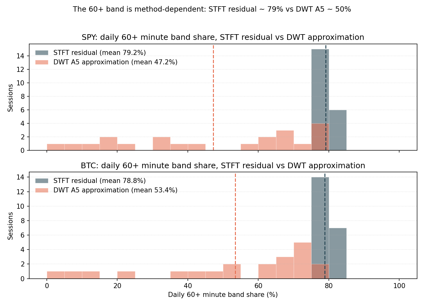
The residual definition for the 60+ band is load-bearing for everything that follows: it absorbs the Hann taper loss at frame edges and any inter-window low-frequency drift, so the 60+ band carries roughly 79% of session variance on this sample. That is partly real low-frequency structure (open/close drift) and partly an artefact of the residual being a catch-all term.

Daily band shares are

The discrete wavelet transform uses Daubechies-4 (db4) with five levels and symmetric boundary handling, following Mallat [1] and Percival and Walden [2]. Detail coefficients $D_1,\dots,D_5$ and the approximation $A_5$ map to bands as

The DWT 60+ band is a genuine wavelet approximation rather than a residual; this is the structural reason the STFT and DWT band-share series disagree at the percentage-point level (Section 5). Sensitivity is reported for boundary modes symmetric (primary), periodic, and zero.

ISO weeks are labelled stress by the union rule

where $\widetilde{\mathrm{VIX}}_w$ is the weekly median VIX close and $\mathrm{RV}^{\mathrm{BTC}}_w$ is the annualized standard deviation of 1-minute BTC log returns within ISO week $w$, computed as $\sigma_w \sqrt{525{,}600}$ (24/7 trading). The 80th-percentile cut on BTC realized volatility is taken over the available weekly panel.

Two complementary Kolmogorov–Smirnov tests are run against daily band-share series, both with a Bonferroni correction across the four bands ($\alpha_{\text{corr}} = 0.05/4 = 0.0125$):

• Stress vs. calm, per asset, per method: $D^{i,b}_{\text{sc}} = \sup_x \bigl|\widehat{F}_{i,b,\,\mathbb{S}=1}(x) - \widehat{F}_{i,b,\,\mathbb{S}=0}(x)\bigr|.$
• Cross-asset, per method: $D^{b}_{\text{x}} = \sup_x \bigl|\widehat{F}_{\mathrm{SPY},b}(x) - \widehat{F}_{\mathrm{BTC},b}(x)\bigr|.$

Because $n = 21$ paired trading days has near-zero power for a distributional test, the report leans on point estimates with nonparametric confidence intervals. For each band $b$ and each bootstrap iteration $k = 1, \dots, B$, paired-day indices are resampled with replacement in contiguous blocks of length $L$, yielding $n$ resampled days; the bootstrap statistic is

Block resampling preserves the joint $(SPY, BTC)$ daily distribution and a coarse amount of serial dependence across adjacent days, which is the dependence structure relevant for spectral statistics. The report uses $L = 5$ trading days (one calendar week), $B = 2000$ resamples, and a fixed random seed. The block-bootstrap construction follows Künsch [4].

This section reports the strongest single finding in the report and is deliberately placed before the cross-asset results, because the cross-asset story cannot be read without knowing how method-dependent it is.

Figure 2 contrasts the daily 60+ minute band share under the two decompositions. The STFT residual concentrates near 79% with a tight right tail; the DWT A5 approximation spreads from roughly 0% to 85% with a mean near 50%. The two histograms are computed on identical input series. Because the four band shares sum to one by construction, a 30-percentage-point shift in the 60+ band must be redistributed across the lower-frequency bands, which is exactly what propagates into the cross-asset comparison.

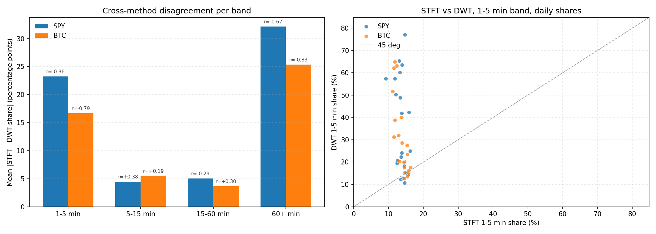
Per-asset, per-band correlations between the STFT and DWT daily share series are reported in Table 1 and visualised in Figure 3. The two methods disagree at the 4–32 percentage-point level on identical inputs, and the daily series are negatively correlated in three of four SPY bands and two of four BTC bands. The 1–5 minute and 60+ minute bands show the strongest negative correlations.

Asset	Band	$|\Delta s|$ (pp)	$r$
SPY	1–5 min	23.23	-0.36
SPY	5–15 min	4.45	0.38
SPY	15–60 min	5.03	-0.29
SPY	60+ min	32.16	-0.67
BTC	1–5 min	16.65	-0.79
BTC	5–15 min	5.48	0.19
BTC	15–60 min	3.65	0.30
BTC	60+ min	25.37	-0.83

The negative correlation is not random; it is a structural artefact of the residual construction. When a session has strong intra-window oscillation in the 5–15 minute band, the STFT captures that energy in the corresponding band power and the 60+ residual shrinks because more of the within-session variance has been accounted for. The DWT A5 approximation, by contrast, measures low-frequency energy directly: its 60+ estimate is largely insensitive to how much energy is captured at higher levels of detail. As a result, days that are “louder” in the 5–15 minute band drive the STFT 60+ down while leaving the DWT 60+ roughly unchanged, producing a $\sim\!-0.7$ correlation by construction. The same mechanism flips signs on the 1–5 minute correlation: days where the STFT captures a lot of 1–5 minute energy will inflate the STFT 1–5 share but tighten the 60+ residual, with no comparable mechanism in DWT.

This subsection does not introduce a new estimate, but it does change how the headline gap should be read. The +0.16 pp gap reported in Section 1 is a property of the STFT 30-minute specification. Under DWT with symmetric boundary handling the same gap is $-6.07$ pp; under DWT with zero padding it is $+0.45$ pp. The qualitative conclusion of the report therefore depends on the decomposition, and the cross-asset result that follows must be read with the methodological caveat in mind.

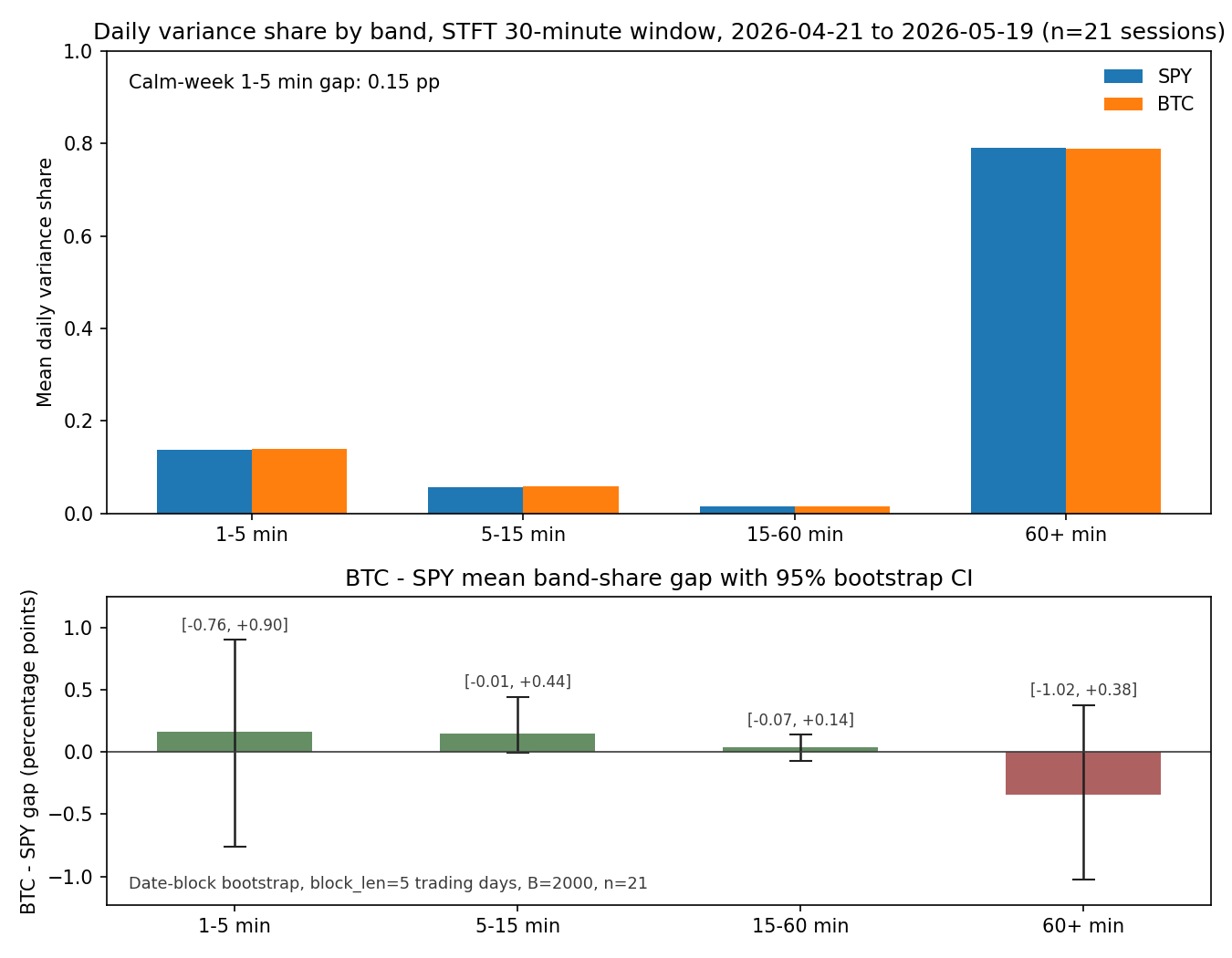
Table 2 reports the BTC-minus-SPY daily mean gap per band, with the date-block bootstrap CI and the share of resamples on which the bootstrap distribution crossed zero relative to the point estimate. All four 95% intervals straddle zero; the 1–5 minute interval includes zero comfortably, and its bootstrap distribution crosses zero on $45.9\,\%$ of resamples. Figure 4 visualizes the level shares (top panel) and the gap with bootstrap brackets (bottom panel).

Band	Point (pp)	CI low	CI high	Crosses zero (share)
1–5 min	0.16	-0.76	0.90	0.46
5–15 min	0.15	-0.01	0.44	0.03
15–60 min	0.04	-0.07	0.14	0.24
60+ min	-0.35	-1.02	0.38	0.21

The 5–15 minute interval narrowly excludes zero ($\text{CI} = [-0.01, +0.44]$) and is the only band where the bootstrap crosses-zero share is small ($3.4\,\%$); it is the closest the data comes to a defensible cross-asset gap on this window. The 5–15 minute band corresponds to periods of roughly six to ten minutes, the time scale at which institutional order-flow batching (VWAP and algorithmic execution cadences) typically shows up in equity intraday variance. A speculative reading is that BTC, traded continuously across venues without that cadence, has a slightly more even distribution of energy across mid-frequencies than SPY, which puts a small extra weight on the 5–15 minute band. The reading is speculative because the cross-asset KS test for the same band is non-significant on this sample.

Table 3 reports the SPY-vs-BTC distributional tests. No band's $p$-value crosses the Bonferroni-corrected threshold under either decomposition.

Method	Band	$D$	$p$ (uncorrected)
STFT	1–5 min	0.190	0.853
STFT	5–15 min	0.238	0.603
STFT	15–60 min	0.238	0.603
STFT	60+ min	0.238	0.603
DWT	1–5 min	0.286	0.365
DWT	5–15 min	0.143	0.987
DWT	15–60 min	0.238	0.603
DWT	60+ min	0.238	0.603

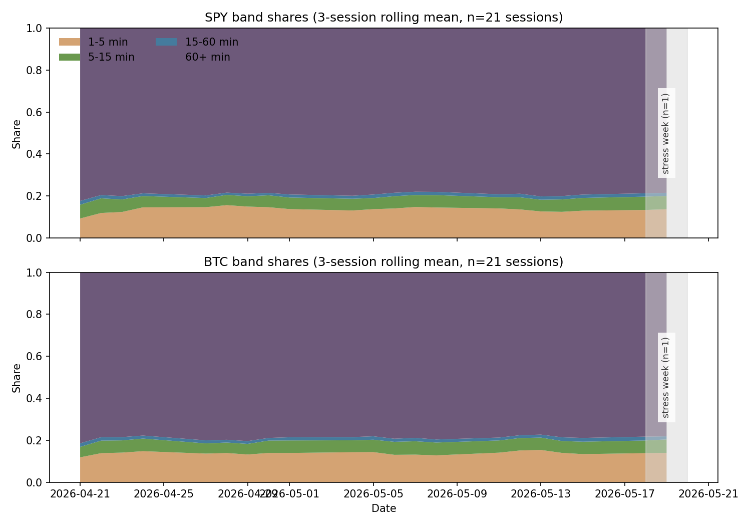
Figure 5 traces the daily band shares per asset across the 21-day window, with adaptive smoothing matched to the sample size and the single ISO stress week shaded.

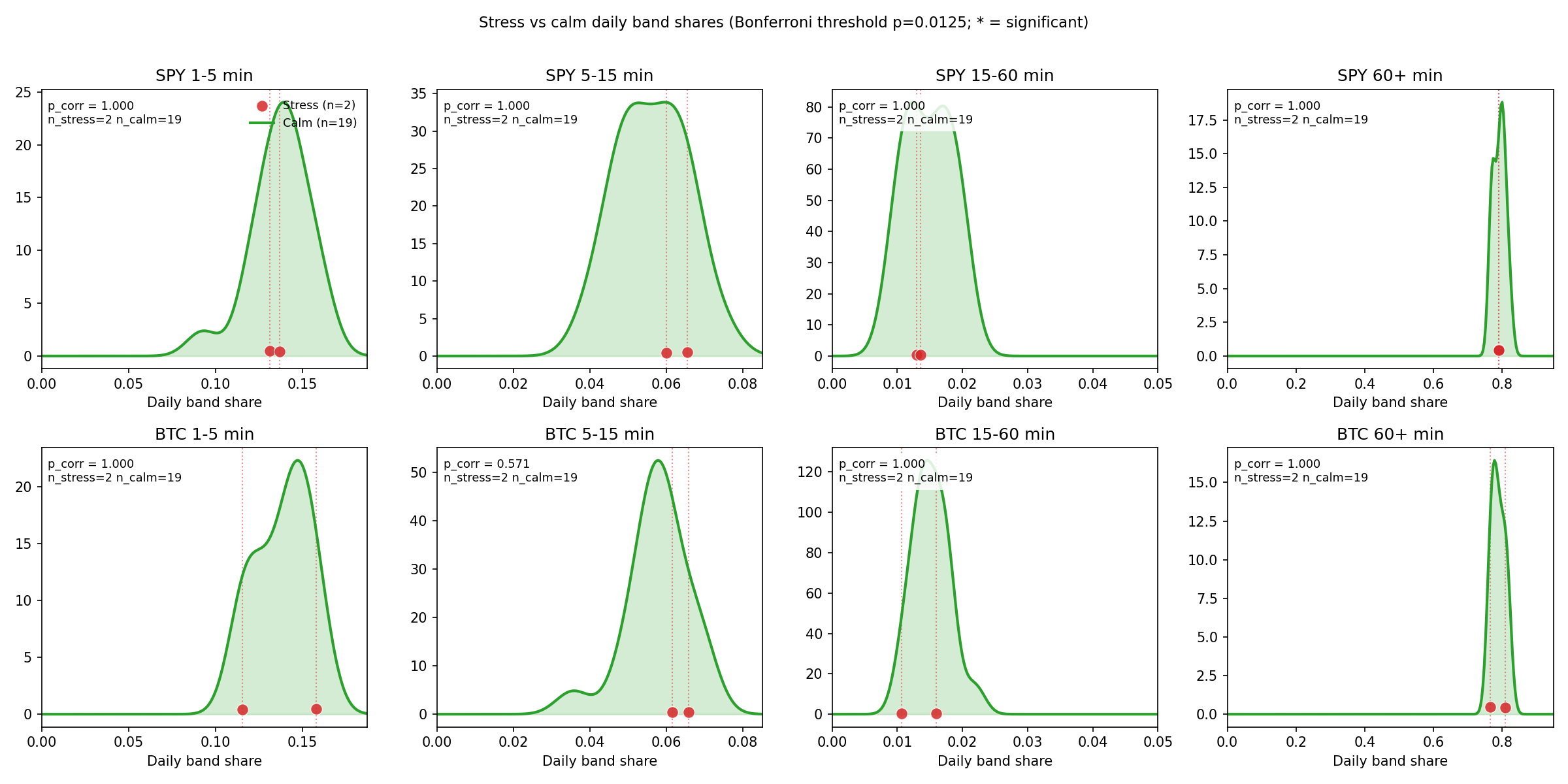
With only two stress-session observations per asset the stress arm is read descriptively. Table 4 shows the calm BTC–SPY gap, the stress BTC–SPY gap, and the stress-minus-calm gap change. The 1–5 minute gap widens by $+0.13$ pp in the stress week; the other bands move in modest opposite directions. None of the stress-vs-calm KS statistics survives Bonferroni correction (the smallest corrected $p$ is $0.57$ for the BTC 5–15 minute band). The headline of $+0.16$ pp is the unconditional 21-day mean; conditioning on calm sessions produces $+0.15$ pp and conditioning on the two stress sessions produces $+0.28$ pp. The full-sample value should be read as the defensible point estimate; the calm/stress decomposition is a diagnostic.

Band	Calm gap (pp)	Stress gap (pp)	Stress $-$ calm (pp)
1–5 min	0.15	0.28	0.13
5–15 min	0.15	0.10	-0.05
15–60 min	0.04	0.01	-0.03
60+ min	-0.34	-0.39	-0.05

Figure 6 shows the stress-vs-calm daily band-share distributions per asset and band. With only two stress observations the stress arm is rendered as a strip plot, not a kernel density.

The headline gap is small. Whether one believes it depends on how stable it is across specification choices. This section walks through three sensitivity exercises; the cross-method audit that motivates each of them was established in Section 5.

Three STFT windows are persisted (15, 30, 60 minutes); band shares are recomputed independently for each. Table 5 reports the mean BTC–SPY gap per band per window. The 1–5 and 5–15 minute gaps are stable in sign and roughly stable in magnitude across windows; the 15–60 minute band is structurally zero for $w = 15$ because a 15-minute window cannot resolve a 30-minute period at all.

Window (min)	1–5	5–15	15–60	60+
15	0.15	0.12	0.00	-0.28
30 (primary)	0.16	0.15	0.04	-0.35
60	0.14	0.12	0.06	-0.32

The DWT result is markedly more sensitive than the STFT result, and not just in magnitude — the sign of the BTC–SPY 1–5 minute gap flips between the symmetric primary mode and the zero mode. Under symmetric, BTC carries $6.07$ percentage points less variance in the 1–5 minute band than SPY; under zero it carries $0.45$ pp more. The mechanism is the session length: with roughly 390 samples per RTH session and a 5-level db4 decomposition, the symmetric boundary extension wraps the session edges into a mirrored copy whose intra-session high-frequency content spuriously inflates the $D_2$ and (via redistribution) $A_5$ coefficients. Zero padding does not produce that artefact at the session boundary, and periodic mode produces an intermediate result.

Boundary mode	1–5	5–15	15–60	60+
symmetric (primary)	-6.07	1.18	-1.34	6.23
periodic	-0.43	-0.25	0.82	-0.14
zero	0.45	-0.86	0.52	-0.10

Replacing BTC's matched-RTH series with the same BTC sampled over the full 24-hour UTC day collapses the headline gap entirely. Table 7 compares the primary BTC matched-session gap to the BTC-24h-vs-SPY-matched gap, by band. The 1–5 minute gap flips from $+0.16$ pp to $-1.12$ pp; the 60+ minute residual moves by more than $2$ pp in the opposite direction. The matched-session result is therefore partly a property of the truncation: outside U.S. hours BTC carries proportionally more low-frequency variance, and the lift in the high-frequency share inside U.S. hours is a relative shift, not an absolute property of the asset.

BTC sampling	1–5	5–15	15–60	60+
Matched (primary)	0.16	0.15	0.04	-0.35
24h	-1.12	-0.72	-0.24	2.07

The sensitivity matrices test seven specifications across four bands; some entries will flip sign by chance even if no underlying signal is present. The matrices should be read descriptively, not as a battery of independent tests.

This section uses the matched 1-minute return series directly, without spectral aggregation, to characterise the within-session variance pattern that drives the band-share decomposition. Andersen, Bollerslev, Diebold and Labys [3] establish the relevant realized-variance framework for the per-minute treatment.

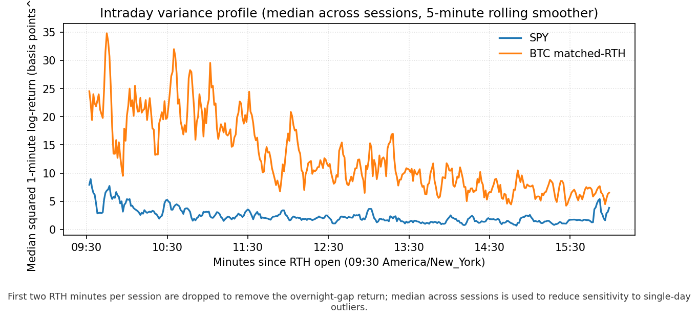
Figure 7 shows the median squared 1-minute log return as a function of minute-of-day, taken across all 21 sessions with the first two RTH minutes per session dropped to remove the overnight-gap return. SPY shows the canonical U-shape — a morning lift, gradual decline through midday, secondary lift into the close. BTC's profile is roughly $5\times$ higher on the same scale, declines through the day more steeply than SPY, and lacks the closing lift, consistent with a 24-hour venue spliced into U.S. hours and lacking the same end-of-day demand for liquidity. The visible intraday non-stationarity is the direct source of the 60+ band's dominance: a falling within-session variance profile is a low-frequency component that the STFT residual absorbs and the DWT A5 represents directly.

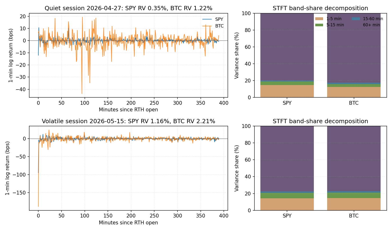
Figure 8 shows two illustrative sessions: the session with the lowest SPY realized volatility on the panel (2026-04-27, RV $\approx 0.35\,\%$) and the highest (2026-05-15, RV $\approx 1.16\,\%$). Both rows display the 1-minute log-return time series and the STFT band-share decomposition. The quiet session is dominated by a single BTC spike near minute 110 that does not register in SPY; the volatile session is more uniformly active across both assets. The band-share decomposition is broadly stable across the two days — both sessions concentrate roughly 80% of variance in the 60+ residual — which underscores that the band shares are a shape statistic, not a level statistic, and a quiet day with one spike can produce a similar band-share decomposition to a uniformly active day.

On a 21-day matched-hours panel SPY and BTC are spectrally near-indistinguishable in the daily distribution of band shares: the 1–5 minute BTC-minus-SPY mean gap is $+0.16$ pp with a bootstrap CI that includes zero by a wide margin, no cross-asset KS test survives Bonferroni correction, and the sign of the gap is not preserved under plausible alternative decompositions. The methodological finding is more durable: the choice between an STFT residual and a DWT approximation for the 60+ minute band moves the cross-asset gap by 5 to 30 percentage points on identical inputs, and the two methods disagree at exactly the bands that drive the headline. The honest reading is therefore narrower than the framing in the original research plan invited: matched-session SPY and BTC do not have visibly distinct spectral signatures at this sample size, and the appropriate follow-up is a longer panel from a paid intraday vendor coupled with a redefinition of the 60+ STFT band as a genuine low-pass filter so the two decompositions can be compared band-for-band without the catch-all term.

1. Sample size. 21 paired RTH trading days. Any distributional test has negligible power on this window; CIs cannot shrink below the bootstrap dispersion driven by individual session variance. The most useful single improvement is extending the SPY intraday history via a paid vendor.
2. Stress conditioning is power-starved. With one ISO stress week and two stress sessions per asset, the stress-vs-calm comparison should be read as a directional diagnostic, not as evidence. A multi-year window will produce a usable stress-week panel.
3. Single-venue BTC. Binance spot BTCUSDT is one of several liquid venues. Cross-venue dispersion in cryptocurrency spot is documented [5]; a composite or an alternative venue (Coinbase, Kraken) is an obvious robustness layer.
4. STFT/DWT band definitions disagree at the 60+ band. The natural next step is to redefine the 60+ STFT band as a genuine low-pass filter rather than a residual, so the two decompositions can be compared band-for-band without the catch-all term. Even with that fix the residual-vs-approximation distinction explains most of the cross-method gap.
5. Extensions. A second asset pair (a major equity index vs. a major altcoin) on the same pipeline, a spectral coherence analysis between SPY and BTC, and the relationship between band-energy shifts and exogenous regime changes are natural follow-ups; all reuse the matched-session return panel as input.

The published artifact set is keyed by a SHA-256 manifest that pins the raw 1-minute SPY and BTC snapshots, the daily VIX series, every processed band-share table (primary and sensitivity), the bootstrap distribution, the Kolmogorov–Smirnov result grid, and the cross-method audit table. The full sample window is 2026-04-21 to 2026-05-19, covering 21 RTH sessions, one ISO stress week, and two stress sessions per asset. The runtime environment is pinned to Python 3.11 with the core scientific stack (numpy, pandas, scipy, pywavelets) and matplotlib for figure rendering; the same manifest hash is produced on two consecutive runs.

References

- Mallat, S. (1989). A theory for multiresolution signal decomposition: the wavelet representation. IEEE Transactions on Pattern Analysis and Machine Intelligence, 11(7), 674–693.
- Percival, D. B. and Walden, A. T. (2000). Wavelet Methods for Time Series Analysis. Cambridge University Press.
- Andersen, T. G., Bollerslev, T., Diebold, F. X. and Labys, P. (2003). Modeling and forecasting realized volatility. Econometrica, 71(2), 579–625.
- Künsch, H. R. (1989). The jackknife and the bootstrap for general stationary observations. Annals of Statistics, 17(3), 1217–1241.
- Makarov, I. and Schoar, A. (2020). Trading and arbitrage in cryptocurrency markets. Journal of Financial Economics, 135(2), 293–319.