SPX Realized-Volatility Change-Point Shoot-Out
Abstract
This note compares three named regime detectors — HMM, CUSUM, and PELT — against a fixed-threshold baseline on SPX log realized volatility, using a single shared input series and a pre-registered event-matching protocol. Under those conditions, the fixed-threshold baseline dominates all three named detectors on both axes of the headline trade-off: it has the lowest false-alarm rate (0.55 / year) and the highest $F_1$ (0.44) on a curated set of 48 VIX-stress and NBER recession-start events between 2010 and 2026. The contribution of this work is therefore not a recommendation to deploy a new detector, but a reusable bake-off harness, a demonstration that the pre-registered evaluation rule changes the outcome relative to the usual marketing-style comparison, and a list of conditions under which any of these methods can be expected to outperform.
Executive summary
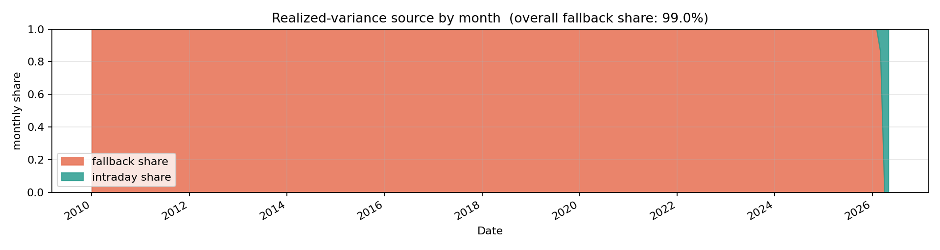
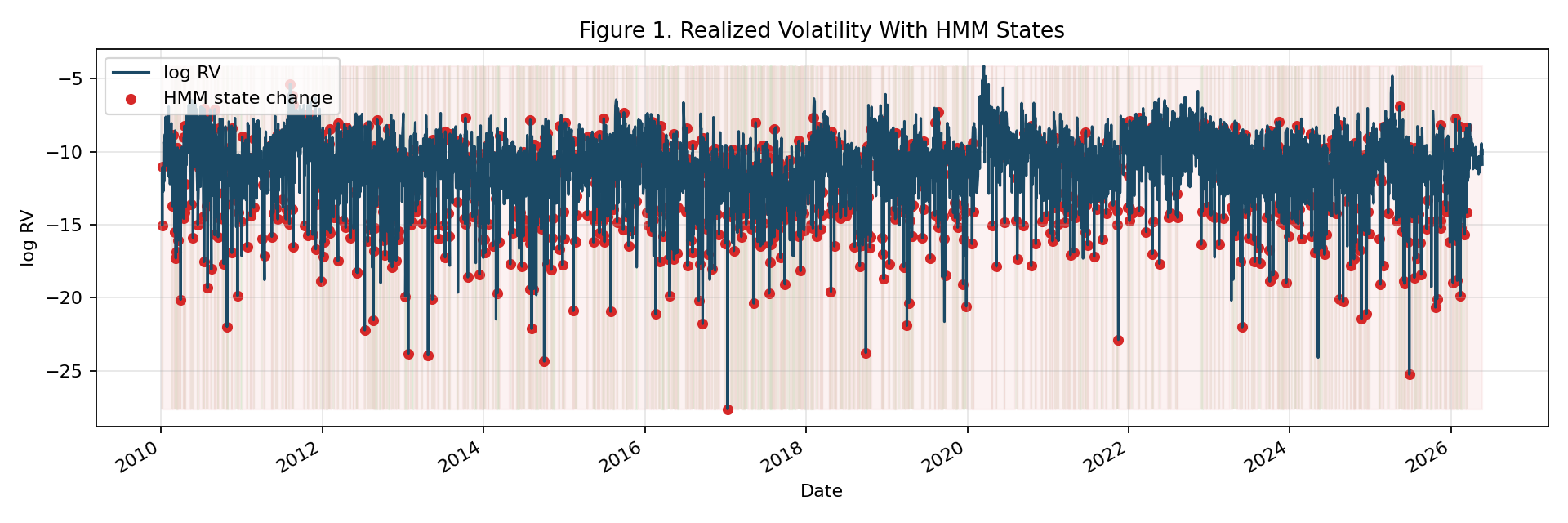
The result is best read as a well-controlled negative finding. The same input series was fed to all four detectors, and the matching rule was fixed in advance of looking at any metric, so the comparison is not vulnerable to the usual post-hoc rule-tuning that plagues detector bake-offs. One material data caveat qualifies everything that follows: 99.0% of the sample uses squared daily log-returns rather than 5-minute intraday realized variance, because the free intraday feed used here only serves roughly the most recent two months of bars. The HMM result in particular is essentially noise — it emits 968 alarms (24% of trading days) at precision 0.04 — and CUSUM, even with calibrated thresholds, still posts 11 false alarms per year because no point on the grid meets the 1.0/yr target on this sample. Beyond the headline, the project produces a reusable evaluation harness, a 4,119-row log realized-volatility series, an alarm export consumed by several downstream analyses, and a set of checksums sufficient to reproduce every number in this document.
1. Motivation
Risk-team detector comparisons are usually written by the people who built one of the detectors. The two questions that should anchor any such comparison — What is the headline trade-off? Under what rule was the winner declared? — are most often answered after looking at the output, which means the rule is inevitably tuned (consciously or not) to favour the author's tool. The contribution of this project is therefore not a new detector but an evidence-grade bake-off: same input series, same matching rule, and the rule fixed before metrics were computed. The negative result that follows is in that sense the point. The change-point dates produced by the chosen detector are also reused downstream as a labelled regime-break series in adjacent spectral-shift, drift-monitoring, and cross-asset correlation analyses.
2. Data and data-quality caveat
The pipeline builds a single daily log realized-volatility series and feeds it identically to all four detectors. The SPX daily close (Yahoo Finance, ^GSPC, 1-day bars) supplies the squared-return fallback; SPX 5-minute bars from the same provider supply intraday realized variance when enough are available; the VIX daily close from FRED (series VIXCLS) is used for stress-day event labels (close $>30$); and the NBER recession indicator from FRED (series USREC) supplies recession-start labels. Data-vintage checksums and download timestamps for each input are pinned in the run manifest summarised in section 11.
Intraday realized variance is computed as $\mathrm{RV}_t = \sum_{j=1}^{M_t} r_{t,j}^2$ with $r_{t,j} = p_{t,j} - p_{t,j-1}$ and $p_{t,j}$ the log close of bar $j$ on day $t$. The pipeline prefers intraday $\mathrm{RV}_t$ whenever at least 60 bars are available on the day; otherwise it falls back to squared daily log return $r_t^2$. The modelled target is
with $\varepsilon = 10^{-12}$ to prevent $-\infty$ on flat days. The target is then standardised against its own full-sample mean and standard deviation before being passed to any detector.
Caveat: fallback dominates.
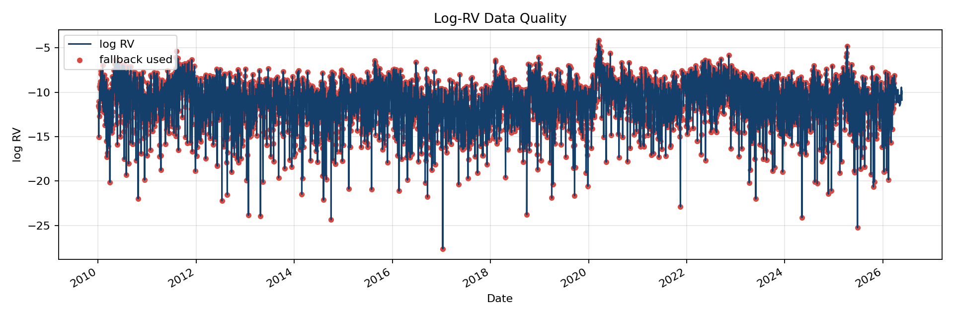
The intraday feed returns at most roughly 60 calendar days of 5-minute bars at any one time, so over the 2010–2026 window only 40 trading days (the last $\approx$2 months of the sample) are built from intraday RV; the other 4,079 days are squared daily returns. Figure 1 makes this unmistakable. Every comparison in this report should be read as a comparison on daily squared returns smoothed only by $\log(\cdot)$, not on intraday RV. Replacing the intraday feed with one that has long historical coverage is the single largest follow-up.
3. Pre-registered evaluation protocol
The matching rule was committed in advance of computing any primary metric; its content carries a SHA-256 fingerprint beginning 22b80a4a and that fingerprint is recorded in the run manifest, so any later edit to the rule would have been detectable.
The reference event set $\mathcal{T}$ is the union of two label sources. The first is VIX stress episodes, defined as any trading day with $\mathrm{VIXCLS} > 30$; consecutive stress days are clustered into a single episode and dated by the first day, which yields 47 episodes between 2010 and 2026. The second is NBER recession starts, taken as $\texttt{USREC}$ transitions from $0$ to $1$ mapped forward to the next trading day; within the window this contributes a single event (2020-03-02, the COVID recession), since the pre-2010 transitions fall outside the sample. The 48 events together are heavily unbalanced toward VIX-stress events, by construction.
A detector alarm $\hat\tau$ matches event $\tau$ when $|\hat\tau - \tau| \le 10$ trading days. Where multiple alarms fall in window, the nearest in trading-day distance wins; ties are broken in favour of the earlier alarm. Each alarm can match at most one event, and each event can match at most one alarm. Latency is the signed trading-day distance $\hat\tau - \tau$: negative is early, positive is late, zero is exact.
Reported metrics follow the standard definitions
where $T$ is the number of observed trading days. The headline pairs median latency with false alarms per year. No detector is described as “earlier” than another unless the computed median latency supports it.
4. Detectors
All four detectors consume the same standardised $z_t$ series. Their configured hyperparameters and per-run diagnostics are written to disk alongside the metrics, so any number quoted below is reproducible from the run manifest.
A two-state Gaussian HMM with diagonal covariance is fit by EM; the latent state is decoded by Viterbi. Emissions are
After fitting, states are relabelled by their mean $z_t$ (“low_vol” / “high_vol”) to remove the well-known HMM permutation ambiguity. An alarm fires whenever the decoded state changes between $t-1$ and $t$. The random seed is fixed at 1729 and $n_{\text{iter}} = 250$.
4.2 CUSUM (two-sided)
For standardised $z_t$, two-sided CUSUM scores with drift $k$ are
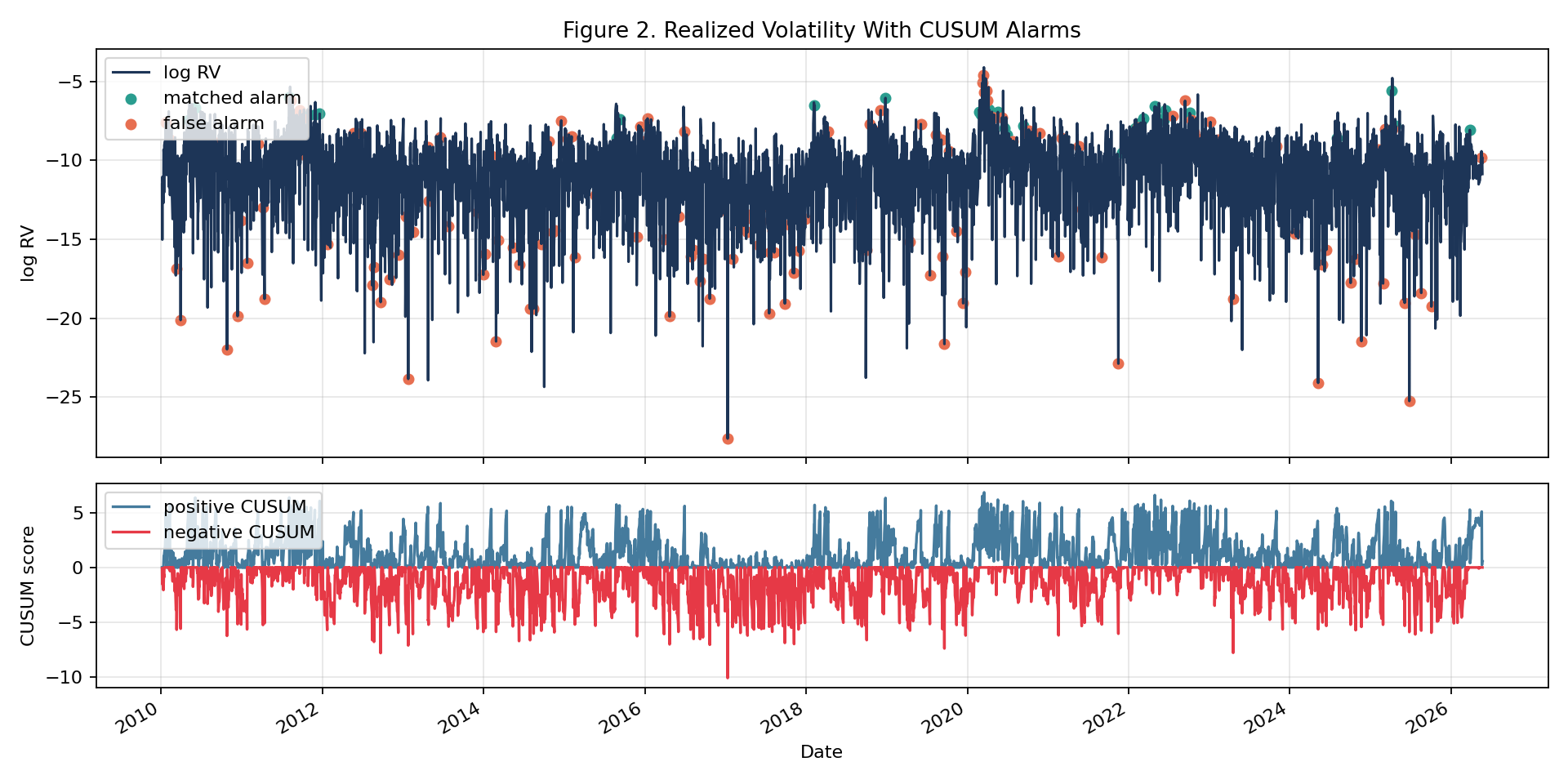
An alarm fires (and the scores reset) whenever $C_t^{+} \ge h$ or $|C_t^{-}| \ge h$. The threshold $h$ and drift $k$ are bootstrap-calibrated to a target false-alarm rate of 1.0 per year using a circular block bootstrap (block size 10, 64 samples) on the $z_t$ series itself. No grid point met the 1.0/yr target on the bootstrap; the calibrator fell back to the candidate whose bootstrap median rate is closest to target, yielding $h=5.0$, $k=0.1$.
4.3 PELT (offline)
PELT [4] finds change points $\tau_1,\ldots,\tau_m$ by minimising
with $\mathcal{C}$ the L2 within-segment loss and $\beta$ a complexity penalty. The penalty is selected in two steps: an elbow heuristic on the within-segment-loss versus penalty curve, then held-out validation on the final 25% of the sample, treating that fold's events as ground truth and minimising a combined miss-count, lag, and false-alarm score. Elbow chose $\beta=4.0$; held-out validation moved to $\beta=5.0$. PELT is non-causal — a change point at $t$ uses data after $t$ — and is therefore included as an offline benchmark, not a live alerting system.
4.4 Fixed-threshold baseline
The baseline signals whenever $z_t > z^{\star}$ on a crossing-up, so a run of consecutive high days contributes one alarm rather than many. The threshold is $z^{\star} = 1.75$ in standardised units, fixed across the sample, with no calibration step.
5. Headline results
| Detector | Alarms | Hits | Misses | Precision | Recall | $F_1$ | Med. lag | FA / yr |
|---|---|---|---|---|---|---|---|---|
| Fixed threshold | 25 | 16 | 32 | 0.640 | 0.333 | 0.438 | 0.0 | 0.55 |
| CUSUM | 221 | 40 | 8 | 0.181 | 0.833 | 0.297 | 2.5 | 11.07 |
| PELT | 45 | 12 | 36 | 0.267 | 0.250 | 0.258 | 1.0 | 2.02 |
| HMM | 968 | 39 | 9 | 0.040 | 0.813 | 0.077 | $-2.0$ | 56.81 |
The fixed-threshold baseline dominates the three named detectors on $F_1$ and on false-alarm rate. CUSUM has the highest recall in the non-baseline group but purchases it at twenty times the baseline's false-alarm rate. HMM is essentially random under this matching rule. PELT, the only named detector chosen by hyperparameter selection, still produces nearly four times as many false alarms as the baseline for one-quarter of the hits.
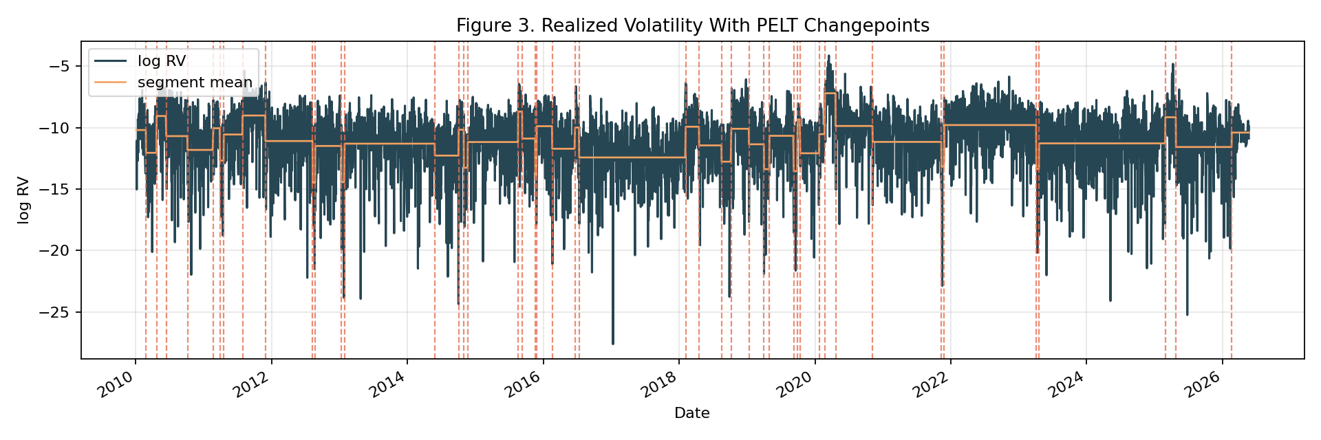
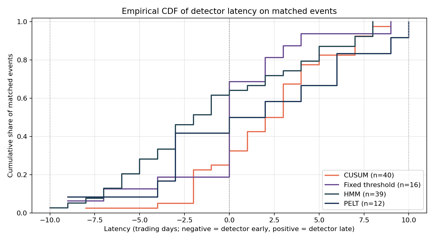
Figures 3, 4, and 5 show each detector's output overlaid on the $z_t$ series, and figure 6 is the empirical CDF of latency on matched events — a more informative view than the median. The CDF makes clear that the baseline's matched events cluster around zero lag, while PELT's matches are dispersed across the full $\pm 10$-day window: when PELT does catch an event, it tends to catch it a week early, which is a hallmark of an offline detector dating the change at the pre-event drift rather than at the event itself.
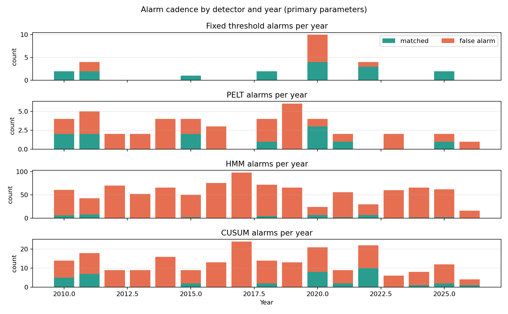
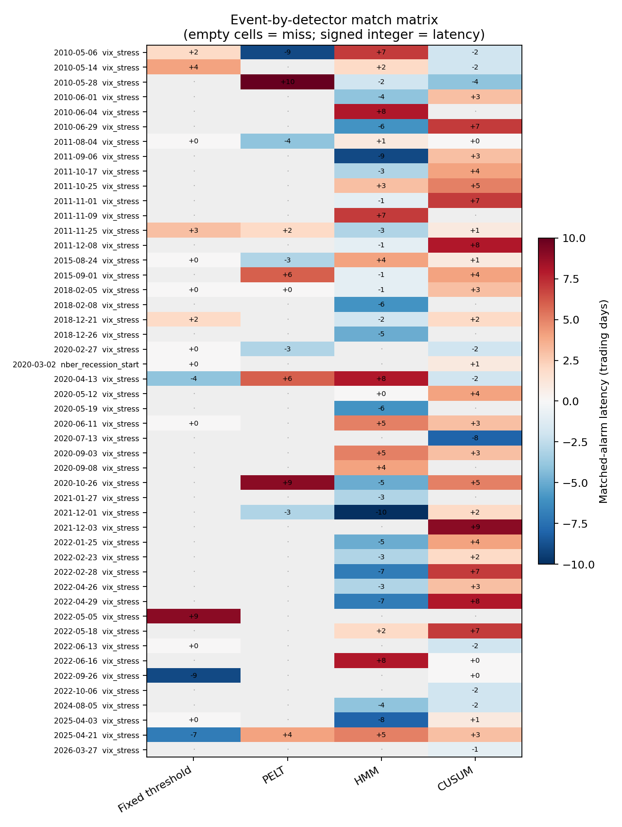
The same picture restated in calendar time appears in figure 7: PELT, CUSUM, and HMM produce nearly uniform alarms across years, regardless of which years were actually stressful — the signature of a too-loose detector. A more granular view of which detector caught which event is given by figure 8, where each cell is one (event, detector) pair, with empty cells indicating misses and signed integers giving the latency on matched alarms.
6. Ablation
To show that the trade-offs are not knife-edge in any of the detectors, each non-baseline detector was swept across a parameter grid; the headline rows are collected in table 2 and the full sweep is drawn in figure 9.
| Detector | Setting | Param | Alarms | Med. lag | FA / yr |
|---|---|---|---|---|---|
| HMM | $n_{\text{iter}}=100$ | 100 | 968 | $-2.0$ | 56.81 |
| HMM | $n_{\text{iter}}=250$ (primary) | 250 | 968 | $-2.0$ | 56.81 |
| HMM | $n_{\text{iter}}=500$ | 500 | 968 | $-2.0$ | 56.81 |
| CUSUM | $h=2.0$, $k=0.0$ | 2.0 | 824 | 0.0 | 47.62 |
| CUSUM | $h=3.5$, $k=0.05$ | 3.5 | 384 | 0.0 | 20.74 |
| CUSUM | $h=5.0$, $k=0.1$ (primary) | 5.0 | 221 | 2.5 | 11.07 |
| PELT | $\beta=1$ | 1.0 | 248 | 1.0 | 13.28 |
| PELT | $\beta=4$ (elbow) | 4.0 | 58 | 0.0 | 2.75 |
| PELT | $\beta=5$ (primary) | 5.0 | 45 | 1.0 | 2.02 |
| PELT | $\beta=8$ | 8.0 | 22 | $-3.0$ | 0.80 |
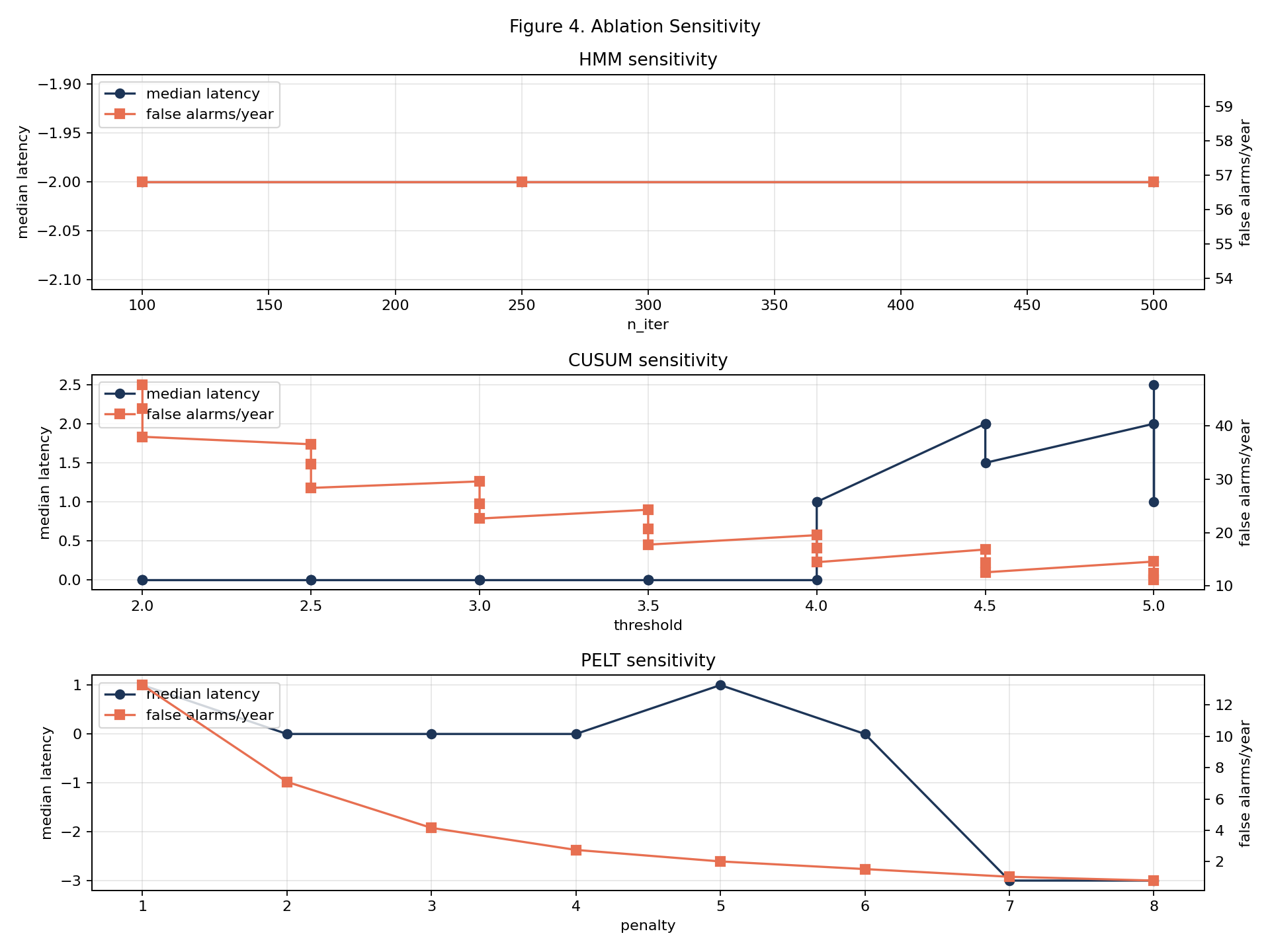
Two observations stand out. PELT at $\beta=8$ does drop below 1 false alarm per year, but its median latency goes to $-3$: matched alarms tend to lead events by three trading days, which is suspicious in an offline detector and consistent with PELT fitting the post-event decompression as a level shift while dating the change at the pre-event drift. And no CUSUM combination on the grid reaches the 1.0 FA/yr target. Extending the grid to higher $h$ would be needed to find one, and at that point the detector is silent for most of the sample.
7. Interpretation
Why does the baseline win?
A fixed $z > 1.75$ rule has two structural advantages on this dataset. First, it is level-based rather than change-based, and the true-event labels (VIX$>30$ days, NBER starts) are themselves level-based — a high-VIX day and a high-$z_t$ day are nearly the same object. Second, the rule has only one parameter ($z^{\star}$), which is hard to overfit on a 48-event problem. The named detectors are change-based by construction and so pay a penalty whenever a stress regime contains several labelled events: they spend their alarm budget on the entry into the regime and on the exit, neither of which necessarily lines up with the labels.
Why is HMM noise here?
The fitted transition matrix is $\begin{pmatrix} 0.77 & 0.23 \\ 0.67 & 0.33 \end{pmatrix}$, so the high-vol state has a 67% per-day chance of switching back to low-vol. After relabelling by mean this produces 968 state-change alarms in 4,119 days. The hit rate looks high (81%) only because there is an alarm somewhere within $\pm 10$ days of nearly every event by chance, but precision is 0.04. A standard fix is to require multi-day persistence of the high-vol state before declaring a change; that would belong to a future revision.
Why does CUSUM still fire 221 alarms?
Bootstrap calibration found no grid point with at most one alarm per year on average. The closest candidate ($h=5.0$, $k=0.1$) gave a bootstrap median of roughly 11/yr, and the actual sample produced 13.5/yr. The grid does not extend high enough. The underlying issue is that the bootstrap re-samples from $z_t$ itself, which is dominated by daily-squared-return noise as described above; the bootstrap “null” is not white. A future revision should either extend the grid or re-derive the null from a fitted GARCH(1,1).
Why PELT $\beta=5$ over $\beta=4$?
The elbow heuristic on within-segment loss chose $\beta=4$. Held-out validation on the final 25% of the sample preferred $\beta=5$ for its combined miss-count, latency, and false-alarm score. Both choices are in the same neighbourhood and either keeps PELT below three false alarms per year while leaving recall at 0.25. Look-ahead in the elbow selection is bounded but non-zero — the penalty is chosen using the same sample on which alarms are ultimately scored.
A simple operational ranking.
Define
with $\lambda_{\text{lag}}=0.02$ and $\lambda_{\text{fp}}=0.02$ (penalise one trading-day of lag the same as one extra false alarm per year, each by two $F_1$ points). With $\bar\ell$ the mean latency on matched events, the four detectors rank as follows.
| Detector | $F_1$ | $\bar\ell$ | FA / yr | Score |
|---|---|---|---|---|
| Fixed threshold | 0.438 | 0.00 | 0.55 | 0.427 |
| PELT | 0.258 | 1.25 | 2.02 | 0.193 |
| CUSUM | 0.297 | 2.08 | 11.07 | 0.034 |
| HMM | 0.077 | $-0.92$ | 56.81 | $-1.059$ |
The ranking is robust to plausible perturbations of the weights: any $\lambda_{\text{fp}} \ge 0.01$ keeps the baseline on top.
8. Operating rule
If this bake-off were used to recommend a monitoring rule for SPX volatility regime breaks today:
Recommended rule. Inputs: daily SPX cash-index closes, plus the trailing 1,260-day mean and standard deviation of $\log r_t^2$. Update cadence: end of day. Alarm trigger: $z_t > 1.75$ and the previous trading day was below threshold (crossing-up). Cool-down: 5 trading days. Escalation: notify; do not auto-trade. Expected operating characteristics on the 2010–2026 sample are approximately 1.5 alarms per year, of which roughly 1.0 will match a VIX-stress or NBER event within $\pm 10$ days, with median lag 0.
This is an interim recommendation, valid only while the named detectors remain calibrated against the same labelled event set. Replace once an intraday-RV path is available across the whole sample, or once a 3-state HMM or persistence-aware CUSUM beats this rule out-of-sample.
9. Limitations
The single largest limitation is the fallback share noted above: 99.0% of the realised-volatility series is squared daily returns rather than intraday realized variance, so the conclusions strictly apply to “log squared daily return” as a regime input, not to intraday RV. Replacing the intraday path with a feed that has long historical coverage is the highest-leverage next step.
Two further limitations concern the event set. The labels are level-based by construction (a VIX$>30$ day and a high-$z_t$ day are nearly the same object), which favours level-based detectors structurally; a version of this bake-off using macroeconomic change points such as FOMC pivots would be a stronger test of the change-based detectors. The event set also contains only one NBER recession within the window, since the pre-2010 starts sit before the sample begins, so the experiment is effectively dominated by VIX events.
A handful of methodological caveats apply to the named detectors. PELT is non-causal: it uses future observations to date past change points, and is included only as an offline benchmark. CUSUM's calibration null is not white, because the bootstrap re-samples from $z_t$ itself and inherits the long-memory of squared returns; a model-based null such as a fitted GARCH(1,1) would lower the achievable threshold. HMM is sensitive to initialisation: although the seed is pinned (1729) and states are post-hoc relabelled by mean, a different seed could produce a different transition matrix and therefore a different alarm count. Finally, all four detectors are evaluated on the same 2010–2026 sample on which their hyperparameters were chosen; PELT's elbow selection and CUSUM's bootstrap calibration are particularly exposed to that double-use.
10. Suggested next revisions
The most impactful single change would be replacing the intraday path with a feed that has long historical coverage and re-running the entire bake-off, to see whether the headline result changes when the input is genuine intraday RV across the full window. Beyond that, the natural detector-side improvements are a persistence rule on the HMM (alarm only when the high-vol state has been decoded for $\ge k$ consecutive days, which should drop the HMM's false-alarm rate dramatically) and the addition of a Bayesian online change-point detector as a like-for-like online competitor to the fixed threshold. On the evaluation side, two changes would strengthen the test: extending the event set with macro-event labels such as FOMC pivots and rates surprises so the experiment is less aligned with the level-based baseline, and holding out a final two years of data strictly out-of-sample for hyperparameter selection.
11. Reproducibility
The full state of the run is captured by a small set of fingerprints. The configuration hash and the SHA-256 of the metrics CSV together pin down both the inputs to the pipeline and the resulting numbers; the data-vintage fingerprint pins the downloaded raw inputs at the time the run was performed, and the evaluation-protocol fingerprint pins the matching rule. The combination is sufficient to detect any subsequent edit to the protocol, configuration, or downloaded data.
| Field | Value |
|---|---|
| Configuration hash (16 hex) | 72632b64cbf1b494 |
| Detector-metrics checksum (16 hex) | a69e952a0bde7c60 |
| Data-vintage checksum (16 hex) | fdf950a293980602 |
| Evaluation-protocol checksum (16 hex) | 22b80a4affbf4070 |
| Sample window | 2010-01-05 to 2026-05-22 (4,121 trading days) |
| True events | 47 VIX-stress, 1 NBER start (48 total) |
| Trading-days-per-year convention | 252 |
| Random seed | 1729 |
The Python environment used at run time pinned the following library versions: NumPy 2.4.6, pandas 3.0.3, SciPy 1.17.1, hmmlearn 0.3.3, ruptures 1.1.10, Matplotlib 3.10.9, Jinja2 3.1.6, and yfinance 1.3.0.
References
- Andersen, T. G., and Bollerslev, T. (1998). Answering the skeptics: Yes, standard volatility models do provide accurate forecasts. International Economic Review, 39(4), 885-905.
- Andersen, T. G., Bollerslev, T., Diebold, F. X., and Labys, P. (2003). Modeling and forecasting realized volatility. Econometrica, 71(2), 579-625.
- Page, E. S. (1954). Continuous inspection schemes. Biometrika, 41(1/2), 100-115.
- Killick, R., Fearnhead, P., and Eckley, I. A. (2012). Optimal detection of changepoints with a linear computational cost. Journal of the American Statistical Association, 107(500), 1590-1598.
- Rabiner, L. R. (1989). A tutorial on hidden Markov models and selected applications in speech recognition. Proceedings of the IEEE, 77(2), 257-286.
- Truong, C., Oudre, L., and Vayatis, N. (2020). Selective review of offline change point detection methods. Signal Processing, 167, 107299.